Layered Subsurface (Soil over Regolith)

1. Overview

The layered subsurface is an optional alternative to the default groundwater scheme described on the Groundwater Model page. It replaces the three-layer soil column, in which the aquifer sits inside the soil, with a soil-over-regolith column that reaches the depth to bedrock. The water-table rules follow the Noah-MP MMF groundwater scheme (Miguez-Macho et al., 2007).

Model	Switch	Default
HydroPol2D-Python	vertical.subsurface.scheme: layered	legacy
HydroPol2D (MATLAB)	flag_layered_subsurface = 1	0

The default scheme is unchanged. Both models implement the same column, and the MATLAB kernels are checked against Python fixtures (see Groundwater and Recharge Validation).

1.1 Why the layered scheme exists

In the default scheme the soil depth is both the soil and the aquifer. A rising water table shrinks the unsaturated store, and the water that no longer fits is returned to the surface as saturation excess (Section 11 of the Groundwater Model). Where the soil is thin and recharge is high, the table reaches the surface and infiltration stops. City-scale runs showed this over large parts of the domain.

The layered scheme changes two things:

1. the aquifer extends below the soil, through the regolith, to the depth to bedrock;
2. a rising water table fills the empty pore space $\theta_s - \theta$ of the unsaturated layers. The water already held there stays where it is instead of being pushed to the surface.

---

2. Soil Base and Depth to Bedrock

Two depths define the column. Both are measured downward from the ground surface. They mark different things:

Depth	What it marks	Role in the layered column
Soil base	Where soil properties end and regolith begins	Bottom of the three soil slots. Below it, slots use regolith parameters.
Depth to bedrock (DTB)	Where the aquifer ends	Bottom of the whole column (soil plus regolith), capped at max_depth_m (default 50 m).

The aquifer base is therefore

$$z_{\mathrm{base}} = z_{\mathrm{surf}} - \min\left(D_{\mathrm{DTB}},\,D_{\max}\right)$$

and not $z_{\mathrm{surf}} - D_{\mathrm{soil}}$ as in the default scheme.

Example. A cell with a soil base at 1.5 m and DTB at 30 m has soil slots from 0 to 1.5 m and regolith slots from 1.5 to 30 m. With DTB at 80 m, the column stops at the 50 m cap. If DTB is shallower than the soil base, the soil slots are cut at DTB.

Each depth is read from the first source found:

Depth	Sources, first found wins
Soil base	soil-base raster, then the scalar soil_base_depth_m (default 2 m)
Depth to bedrock	DTB raster, then the scalar depth_to_bedrock_m, then the soil depth of each soil class (with a warning)

In the layered scheme the soil depth of the default scheme is used only as this last fallback. The Depth to Bedrock page describes the global data sources for both depths.

---

3. Column Structure

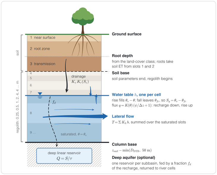
Figure 1. The layered column of one cell (not to scale). The water table splits the slot it is in. The symbols are defined in the table below.

Symbols in Figure 1

Symbol	Meaning	Units
$h$	Water-table head, one per cell	m
$\theta$	Water content of the unsaturated part of a slot	m³/m³
$\theta_s$	Saturated water content	m³/m³
$\theta_r$	Residual water content	m³/m³
$\theta_{fc}$	Water content at field capacity, $\theta(\psi = -3.3\ \mathrm{m})$ by default; also the level up to which capillary rise refills a slot	m³/m³
$S_y$	Specific yield (drainable porosity), $\theta_s - \theta_{fc}$	—
$S_e$	Effective saturation, $(\theta - \theta_r)/(\theta_s - \theta_r)$	—
$K_v$	Vertical saturated hydraulic conductivity of a slot	m/s
$K_r(S_e)$	Mualem–van Genuchten relative conductivity	—
$K(\theta)$	Unsaturated conductivity of a slot, $K_v\,K_r(S_e)$	m/s
$q$	Darcy flux between the lowest unsaturated slot and the water table; positive down (recharge), negative up (capillary rise)	m/s
$\psi$	Matric head of the lowest unsaturated slot; $\psi = 0$ at the water table	m
$\Delta z$	Half the unsaturated thickness of that slot	m
$T$	Transmissivity for lateral flow	m²/s
$K_h$	Horizontal saturated conductivity of a slot, including its lateral multiplier	m/s
$b$	Saturated thickness of a slot	m
$z_{\mathrm{surf}}$	Ground-surface elevation	m
$D_{\mathrm{DTB}}$	Depth to bedrock	m
50 m	Default cap on the column depth, max_depth_m	m
$f_d$	Fraction of the recharge sent to the deep aquifer, deep_recharge_fraction	—
$Q$	Outflow of a deep reservoir	m³/s
$S$	Storage of a deep reservoir	m³
$\tau$	Response time of the deep reservoirs, deep_aquifer_response_time_days	days

Slot	Depth range	Parameters
1. Near surface	$0$ to $l_{\mathrm{top}}$	soil van Genuchten curve, near-surface $K_{\mathrm{sat}}$
2. Root zone	$l_{\mathrm{top}}$ to root depth	soil van Genuchten curve, root-zone $K_{\mathrm{sat}}$
3. Transmission	root depth to soil base	soil van Genuchten curve, transmission $K_{\mathrm{sat}}$
4, 5, … Regolith	soil base to column base	regolith van Genuchten curve, $K_v$, $K_h$

The regolith slots follow a fixed ruler from the soil base: 0.25, 0.5, 1, 2, 4, 4, 4, … m (first thickness 0.25 m, growth ratio 2, maximum 4 m). The ruler is cut at the column base.

Three rules keep the column regular:

• Fixed slot count. Every cell has the same number of slots. Slots below the column base have zero thickness.
• Collapsing slots. Roots shallower than $l_{\mathrm{top}}$ leave slot 2 empty. Roots deeper than the soil base leave slot 3 empty. A slot thinner than 5 mm is merged into the slot above.
• One water table per cell. The head $h$ moves across fixed slot boundaries. It splits the slot it is in into an unsaturated part above and a saturated part below.

3.1 State variables

Variable	Meaning	Units
$h$	water-table head, one per cell	m
$W_k$	water above $\theta_r$ in the unsaturated part of slot $k$	mm
$b_k$	saturated thickness of slot $k$ (below $h$, at $\theta_s$)	m

The water content of the unsaturated part of slot $k$ with unsaturated thickness $u_k$ is

$$\theta_k = \theta_{r,k} + \frac{W_k}{u_k}$$

---

4. Process Rules

4.1 Rising water table

Water added at the table fills the empty pore space of the unsaturated part of the slot that holds the table. A net volume $V$ (per unit area) raises the table by

$$\Delta z = \frac{V}{\theta_{s,k} - \theta_k}$$

The water already in that part of the slot stays there and becomes saturated water, so only the empty pore space $\theta_{s,k} - \theta_k$ has to be filled. This is the water-table rise of the MMF groundwater scheme (Miguez-Macho et al., 2007), which Noah-MP does in its UPDATEWTD routine. The rise moves into the slot above only once the current slot is full, so round-off cannot skip an unfilled slot. Water left over when the table reaches the ground leaves as exfiltration (seepage) to the surface.

4.2 Falling water table

Water removed at the table lowers it. The thickness that the table exposes is left at field capacity, $\theta_{fc} = \theta(\psi = -3.3\ \mathrm{m})$. Each metre of fall therefore releases

$$S_y = \theta_s - \theta_{fc}$$

This is the drainable porosity, with the specific retention taken as field capacity (Lv et al., 2021). The water above $\theta_{fc}$ in the exposed thickness drains later by gravity. A fall and a rise of the same volume are reversible. Removal that cannot be met before the column base is reported as unmet.

The field-capacity head is capillary_field_capacity_head_m (default 3.3 m). Soil slots always take $S_y$ from their own retention curve. Regolith slots do too, unless a regolith $S_y$ is given as a scalar or raster; it must lie in $(0,\ \theta_s - \theta_r]$. A per-slice equilibrium content $\theta_{eq}(z)$ was tested and dropped, because its release tends to zero for thin slices.

4.3 Drainage between slots

Water drains downward through the unsaturated slots under a unit gradient, as in the kinematic unsaturated-zone model UZF1 (Niswonger et al., 2006):

$$q_k = K_{v,k}\,K_r(S_{e,k})$$

with the Mualem–van Genuchten relative conductivity $K_r$. Each flux is limited by the water in the donor slot and by the free space in the next slot below that has an unsaturated part. Fluxes use start-of-step states. The step can be split into drainage_substeps (default 1). The lowest unsaturated slot does not drain by this rule; it exchanges water with the table (Section 4.4).

4.4 Darcy flux at the water table

Between the lowest unsaturated slot and the table, HydroPol2D uses a Darcy flux, positive downward:

$$q = K(\theta_k)\left(\frac{\psi_k}{\Delta z} + 1\right), \qquad \Delta z = \tfrac{1}{2}u_k$$

where $\psi_k$ is the matric head of the slot and $\psi = 0$ at the table. A downward flux is recharge, limited by the slot's water. An upward flux is capillary rise, limited by the drainable water below the table and by the refill rule below.

Capillary refill rule. Capillary rise refills the lowest unsaturated slot only up to field capacity, the water content $\theta_{fc}$ that a falling table leaves behind (where a regolith $S_y$ is given, $\theta_s - S_y$). This is the HBV approach (Lindström et al., 1997). The upward flux therefore stops once

$$\theta_k \ge \theta_{fc}$$

and it never wets the soil above a shallow table toward saturation. The rule holds in HydroPol2D-Python (since fe81252) and in the MATLAB model (since 051b52b), on the structured grid and on the mesh.

Before this rule, capillary rise filled the slot toward hydrostatic equilibrium while a falling table left field capacity behind, so water circulated up and down near a shallow table. In the calibration twin valley:

Measure	Before	After
Water cycling between soil and table, column alone	9.3 × 10⁻³ m³/s	0
Cells flipping flux sign every step, column alone	38	0
Gross capillary rise, full model	0.016 m³/s	0
Stream flow	unchanged	unchanged

The trade-off is that the model has no capillary fringe. To represent one, lower capillary_field_capacity_head_m: $\theta_{fc}$ and $S_y$ then change together.

Implicit flux (default). Over a thin unsaturated gap above a shallow table, the explicit flux is stiff: at long steps it overshoots and flips sign. By default HydroPol2D takes the flux at the end of the step with one linearised backward-Euler step per cell, without iteration:

$$q = \frac{q_0}{1 + \Delta t\,\max\!\left(\dfrac{\partial q}{\partial W} - \dfrac{1}{S_y^{*}}\dfrac{\partial q}{\partial h},\ 0\right)}$$

where $q_0$ is the explicit flux and $W$ is the water of the slot. The derivative with respect to the head follows the move of the table that the flux causes: a rise keeps the gap's water content, and a fall exposes $\theta_{fc}$. $S_y^{*}$ is the storage cost of that move ($\theta_s - \theta_k$ of the gap when water goes down). Only the damping part of the derivative is kept. A saturated gap ($\theta_k = \theta_s$) drains at $K_{sat}$ without damping. CLM5 also solves its water-table flux implicitly. At short steps the two forms agree.

Test: sand, $\theta = 0.41$, table 30 cm deep (nearly saturated gap), 1-h steps, against a 1-s run	Result
Implicit flux	the table stays within 2 mm of the 1-s run
Explicit flux	drains about 20 times too much water

Model	Switch	Derivatives
HydroPol2D-Python	implicit_water_table_flux (default true)	jax.jvp
HydroPol2D (MATLAB)	flag_implicit_water_table_flux (default 1; HYDROPOL_IMPLICIT_WATER_TABLE_FLUX overrides it)	fourth-order central differences

The two models agree to about $10^{-9}$, and their parity tests use a tolerance of $10^{-8}$.

4.5 Lateral flow

Lateral flow uses the Dupuit–Forchheimer approximation with a layered transmissivity:

$$T = \sum_k K_{h,k}\,b_k$$

The face transmissivity is the arithmetic mean of the two cells, and the face flux is $Q = -\bar{T}\,\dfrac{\Delta h}{\Delta x}\,w$ for a face of width $w$. The horizontal conductivity of each slot is

Slots	$K_h$
Soil (1–3)	soil $K_{\mathrm{sat}}$ × soil_lateral_anisotropy × soil_lateral_conductivity_multiplier
Regolith (4, …)	regolith $K_h$ × regolith_lateral_conductivity_multiplier

Both multipliers default to 1. The groundwater recession calibration fits them. If no regolith $K_h$ is given, the groundwater $K_{\mathrm{sat}}$ of the default scheme is used.

Lateral flow advances with explicit substeps limited by

$$\Delta t \le C_{\mathrm{gw}}\,\frac{\min(\Delta x,\Delta y)^2\,S_y}{4\,T}$$

with $C_{\mathrm{gw}}$ = groundwater_courant (default 0.25) and $S_y$ taken at the table. Outflow from a cell is limited by its drainable water. Net volumes go through the rising and falling rules above, so heads, unsaturated water and seepage stay consistent. Fixed-head (Dirichlet) cells keep their head, and their exchange is reported as boundary inflow. Lateral flow runs on the groundwater scheduler (Section 2.1 of the Groundwater Model).

4.6 Root-water uptake

With Feddes stress enabled, soil ET is reduced by $\alpha(h)$ in each rooted layer (Hydrologic Model, Section 3.5). Without Feddes, roots that reach below the water table take the unmet part of the demand from the table. That part is the saturated fraction of the root depth, and it is limited by the drainable water.

4.7 Deep aquifer

When the deep aquifer is active, a fixed fraction of the recharge that reaches the table goes to the deep linear reservoirs instead (Groundwater Model, Section 13).

---

5. Order of Operations

Vertical exchange runs every surface step. Lateral flow runs when the groundwater scheduler is due.

1. Infiltration into the soil slots (the Darcy infiltration of the Hydrologic Model).
2. Open-water evaporation, then soil ET, with optional Feddes stress.
3. Drainage cascade between the unsaturated slots.
4. Darcy flux at the water table: recharge or capillary rise.
5. Split of recharge to the deep aquifer, if active.
6. Water-table update; seepage goes to the surface.
7. River–groundwater exchange, if active.
8. Lateral flow, when the scheduler is due.

On the Voronoi mesh, the HRUs of a cell share its ground, column base and head. Their vertical exchange is summed per cell and applied at the groundwater update, by bisection on the cell's storage curve. Lateral flow uses the area-weighted transmissivity.

The layered scheme also supports river–groundwater exchange on the mesh engines (resolved riverbed cells and Neal channels) and exfiltration from green infrastructure into the soil slots.

---

6. Engines and Speed

Engine	HydroPol2D-Python	HydroPol2D (MATLAB)
Structured grid	core/layered_vertical.py	flag_layered_subsurface = 1
Voronoi mesh	NumPy (voronoi_layered.py) and JAX (mesh_gpu/layered.py); NumPy–JAX parity about $10^{-15}$ relative	Voronoi runner (config.layered_subsurface)

In Python, the structured-grid layered step is compiled once per case. The results are identical to the uncompiled step. Profiling on 2026-10-19 gave:

Measure	Before compiling	After compiling
Layered step, 31 steps	2.9 s	0.09 s
One routed hour	4.6 s	0.7 s

After compiling, the layered scheme runs faster than the default scheme. HYDROPOL2D_LAYERED_JIT=0 runs the step operation by operation as a reference.

Separate soil and groundwater clocks (multi-rate time stepping, as in MIKE SHE, GSSHA, Noah-MP and CLM5) were reviewed and are paused. After compiling, surface routing takes most of the run time, so a separate soil clock would gain little.

---

7. Outputs

Output	Python structured grid	Python mesh	MATLAB	Meaning
Groundwater depth	groundwater_depth_map_m	groundwater_depth_face_m	Maps.Hydro.GWdepth_save	Depth of the table below ground (m), capped at the column base
Column base	column_base_depth_m	column_base_depth_face_m	Maps.Hydro.ColumnBaseDepth_m	$\min(D_{\mathrm{DTB}}, D_{\max})$ below ground (m), static
Root-zone and transmission saturation	root_zone_saturation_map, transmission_zone_saturation_map	—	—	$\theta/\theta_s$ of the unsaturated part of slots 2 and 3; NaN where the slot is saturated
Deep vadose storage	deep_vadose_storage_map_mm	deep_vadose_storage_face_mm	Maps.Hydro.DeepVadose_save	Water above $\theta_r$ in the unsaturated part of the regolith slots (mm)

The saturated thickness is the column base depth minus the groundwater depth. It is not saved. Per-slot rasters and depth slices are not written yet; the per-slot states are kept in the model state and in checkpoints.

---

8. Configuration

HydroPol2D-Python:

vertical:
  feddes: {enabled: true, h1_m: -0.1, h2_m: -0.25, h3_m: -4.0, h4_m: -80.0}
  groundwater_courant: 0.25          # lateral-flow substep safety factor
  capillary_field_capacity_head_m: 3.3
  subsurface:
    scheme: layered
    soil_base_depth_m: 2.0           # or static.soil_base_depth_path
    depth_to_bedrock_m: 20.0         # or static.depth_to_bedrock_path
    max_depth_m: 50.0
    deep_layers: {first_thickness_m: 0.25, growth_ratio: 2.0, max_thickness_m: 4.0}
    regolith_theta_s: 0.35
    regolith_theta_r: 0.05
    regolith_alpha_vg_m_inverse: 2.0
    regolith_n_vg: 1.5
    regolith_ksat_v_mm_h: 5.0
    regolith_ksat_h_mm_h: null       # null: vertical.groundwater_ksat_mm_h
    regolith_specific_yield: null    # null: theta_s - theta_fc of the regolith curve
    soil_lateral_anisotropy: 1.0
    soil_lateral_conductivity_multiplier: 1.0
    regolith_lateral_conductivity_multiplier: 1.0
    implicit_water_table_flux: true
    drainage_substeps: 1

A static.regolith_<name>_path raster wins wherever it is finite. The scalar fills the rest.

HydroPol2D (MATLAB): the Soil and groundwater tab of the case workbook holds every setting above, block by block, with its switch at the top of the block (flag_layered_subsurface, flag_feddes, flag_implicit_water_table_flux). See Case Workbook Settings and Model Flags.

---

9. Known Limits

• No perched lateral flow. A saturated soil slot over unsaturated regolith does not flow laterally.
• No regolith class table. Regolith parameters are scalars or rasters.
• No per-slot raster outputs.
• No capillary fringe. Capillary rise refills a slot only up to field capacity (Section 4.4). Lowering capillary_field_capacity_head_m represents a fringe, with a smaller $S_y$.
• Compiled city loop. The compiled HydroPol2D-Python city loop does not yet run the layered scheme with lateral groundwater flow.
• Two ways to take the implicit derivatives. Python uses jax.jvp and MATLAB uses central differences. They agree to about $10^{-9}$.

---

10. Sources

• Miguez-Macho, G., Fan, Y., Weaver, C. P., Walko, R., and Robock, A. (2007). Incorporating water table dynamics in climate modeling: 2. Formulation, validation, and soil moisture simulation. Journal of Geophysical Research, 112, D13108. doi:10.1029/2006JD008112
• Noah-MP, GroundWaterMmfMod.F90.
• Niswonger, R. G., Prudic, D. E., and Regan, R. S. (2006). Documentation of the Unsaturated-Zone Flow (UZF1) Package for modeling unsaturated flow between the land surface and the water table with MODFLOW-2005. USGS Techniques and Methods 6-A19. pubs.usgs.gov/tm/2006/tm6a19
• Lv, M., et al. (2021). A comprehensive review of specific yield in land surface and groundwater studies. Journal of Advances in Modeling Earth Systems, 13, e2020MS002270. doi:10.1029/2020MS002270
• Feddes, R. A., Kowalik, P. J., and Zaradny, H. (1978). Simulation of Field Water Use and Crop Yield. Pudoc, Wageningen.
• Lindström, G., Johansson, B., Persson, M., Gardelin, M., and Bergström, S. (1997). Development and test of the distributed HBV-96 hydrological model. Journal of Hydrology, 201, 272–288. doi:10.1016/S0022-1694(97)00041-3