Calibration Against Observations

This calibration fits model parameters to several kinds of observations at once: discharge, water depth, water level and groundwater depth. Every candidate is a full model run of the event, scored against every observed series. Two search methods are available: a genetic algorithm (GA) that follows the MATLAB GenericGA (the default), and SCE-UA, the shuffled complex evolution of the University of Arizona. The user chooses which parameters are free; the others keep the model's values. In HydroPol2D Studio it is the Calibrate workspace.

The two calibration tools answer different questions:

Tool	Data	Fits
This page	Observed series during an event or period: discharge, depths, water levels, wells	Any parameter of the model, chosen by the user
Groundwater recession calibration	Long daily discharge records, through their master recession curve	Aquifer conductivity and storage, and the starting groundwater state

The calibrated values are effective parameters for this model structure and these data. They are not measurements of the soil or the aquifer.

---

1. Observations

Each observed series is a target. A target has a kind, a place where the model is compared with it, and its own score.

Kind	Compared with
Discharge	A routing gauge, or the model outlet (all boundary outflow)
Water depth	A routing gauge (the mean of its cells), an observation point, or the cell at the series' coordinates
Water level (stage)	As water depth, in the same datum as the terrain
Groundwater depth	An observation point, or the cell at the series' coordinates

• Times are in minutes from the start of the run. The model output is interpolated to the observation times.
• A warm-up period is simulated but not scored. Observations before it are ignored.
• Changes only removes each series' mean before scoring. It is meant for wells whose datum is uncertain and for depths whose bed level comes from the DEM. The ups and downs count, and a constant offset does not.
• Uncertainty (optional) is the measurement error of each value, as one standard deviation in the value's units. Section 2.3 explains how it is used.

Observations are recorded at observation points, which are not yet available on Voronoi and quadtree meshes. On a mesh, only discharge at routing gauges can be calibrated.

---

2. The Score

2.1 One error per series

Each series gets an error $E$ that has no units and is 0 for a perfect fit, so that discharge, depths and well levels can be added. With $s_i$ the simulated and $o_i$ the observed values:

Score	Error $E$	Default for
KGE	$\sqrt{(r-1)^2 + (\alpha-1)^2 + (\beta-1)^2}$	Discharge, water depth, groundwater depth
NSE	$\sum (s_i - o_i)^2 \,/\, \sum (o_i - \bar o)^2$	Water level
NSE of log values	as NSE, on $\ln(x + \bar o/100)$; favours low flows
RMSE / std	$\mathrm{RMSE} / \sigma_o$
Peak, volume and timing	the HydroPol2D GenericGA hydrograph score (below)
Error / uncertainty	$\sqrt{\tfrac{1}{n}\sum \left((s_i - o_i)/u_i\right)^2}$

In KGE (Gupta et al., 2009), $r$ is the correlation, $\alpha = \sigma_s/\sigma_o$ the ratio of standard deviations and $\beta = \bar s/\bar o$ the ratio of means; $E = 1 - \mathrm{KGE}$. NSE is the efficiency of Nash and Sutcliffe (1970); $E = 1 - \mathrm{NSE}$. Water levels and heads use NSE by default because their datum is arbitrary, and the KGE ratio of means says little about a level of 500 m. With Changes only, KGE drops its bias term.

The peak, volume and timing score is the composite of the MATLAB GenericGA:

$$E = \frac{\mathrm{RMSE}}{Q_p} + \frac{|V_s - V_o|}{V_o} + 0.75\,\frac{|Q_{p,s} - Q_p|}{Q_p} + 0.25\,\frac{|t_{p,s} - t_p|}{7200\ \mathrm{s}} + 0.25\,\frac{|\bar s - \bar o|}{Q_p}$$

where $Q_p$ and $t_p$ are the observed peak and its time, and $V$ is the volume over the scored window.

2.2 One score for the calibration

The calibration minimizes the weighted mean of the errors:

$$J = \frac{\sum_e \omega_e \sum_k w_k E_k}{\sum_e \omega_e}, \qquad \sum_k w_k = 1$$

where $e$ runs over the simulated events and $k$ over the series of each event. Without explicit weights, each kind of observation gets an equal share, split equally among its series: with one discharge gauge, one depth gauge and two wells, the weights are 1/3, 1/3, 1/6 and 1/6. Ten wells therefore do not outweigh one discharge gauge. Depth and water level count as one kind, and so do groundwater depth and head. When the user gives a weight to any series, series without one count as 1 and all weights are normalized.

2.3 Using the uncertainty

With Use uncertainty, each point counts with the weight

$$w_i = \frac{u_i^{-2}}{\sum_j u_j^{-2}},$$

so the most uncertain values matter least. Means, variances, the correlation and the residual sums of KGE, NSE, log NSE and RMSE / std then use these weights. With the same uncertainty everywhere the scores do not change. Values without an uncertainty take the median of the known ones. The peak, volume and timing score ignores the uncertainty.

The error / uncertainty score uses it directly. A value of 1 means the model misses by one measurement error on average; below 1 it fits within the data's own error. The results also give the share of points within $\pm u_i$.

---

3. Parameters

Every parameter the model can calibrate is listed, and each is either free or fixed. Fixed parameters keep the model's values. The list follows the active modules and the subsurface scheme: a case without snow has no snow parameters, and a layered case has no single specific yield, because there $S_y$ comes from each slot's retention curve.

A parameter is one of three things:

Kind	Example	What changes
A multiplier on a model field	Manning n × 1.3	The configuration value, every class row and the raster, all multiplied, so the map keeps its pattern
A value of one class	Manning n of land cover 2	That class row
A single value	Regolith lateral conductivity multiplier	That configuration value

A field multiplier gives exactly the factor times the prepared map, whichever input supplied each cell. Start with them. A few multipliers can be identified where many class values cannot. Bounds are on a log scale for conductivities, roughness and other positive factors, and linear for fractions.

Group	Parameters
Surface	Manning n, depression storage, channel Manning n (subgrid channels)
Soil and infiltration	Saturated conductivity, van Genuchten α and n, θs, θr, soil depth
Evapotranspiration and canopy	Root depth, crop coefficient, Feddes heads h3 and h4, canopy storage per LAI
Groundwater	Specific yield and groundwater conductivity (default scheme), riverbed conductivity, capillary field-capacity head, vertical anisotropy
Layered subsurface	Soil and regolith lateral-conductivity multipliers, soil lateral anisotropy, regolith properties, soil base depth, depth to bedrock
Deep aquifer	Deep recharge fraction, response time, initial deep baseflow
Snow	Degree-day factor, all-snow and all-rain temperatures, albedo, fresh-snow density
Water quality	Buildup maximum and rate, washoff coefficient and exponent, antecedent dry days
Initial state	Initial soil water content, initial water-table depth

Every candidate is checked by the model's own rules before it runs. A candidate with $\theta_i > \theta_s$, or with Feddes heads out of order, is refused and gets the worst score.

---

4. The Search

Both methods work on the free parameters in their search scale (log or linear), start from the same kind of sample, and use the same scores, parallel runs, saved runs and result files. They differ in how they choose the next candidates.

4.1 SCE-UA

SCE-UA (Duan et al., 1992; 1993) combines a local simplex search with a global exchange of information:

1. Starting sample. $p \times m$ points spread evenly over the bounds (a Latin hypercube), with the current model as one of them, each scored with a full model run.
2. Deal into complexes. The points are sorted by score and dealt into $p$ complexes of $m$ points, like cards, so that every complex holds good and poor points.
3. Evolve each complex. A complex picks $q$ of its points, favouring the better ones, and tries to replace the worst of them. It first reflects the worst point through the centroid of the others. If that is not better, it contracts halfway toward the centroid. If that fails too, it takes a random point in the smallest box that holds the complex. A complex makes $\beta$ such steps.
4. Shuffle. The complexes are merged and sorted, and dealt again, so that what one complex found reaches the others.
5. Repeat until a stop rule is met.

Setting	Default	Meaning
Complexes $p$	the number of free parameters $n$, at least 2	More complexes search more widely, and run more models at once
Points per complex $m$	$2n + 1$
Simplex size $q$	$n + 1$	Points that take part in one step
Evolution steps $\beta$	$2n + 1$	Steps of each complex between shuffles
Maximum runs	1000	Checked between shuffles
Stop on improvement	below 0.1 % within 5 shuffles
Stop on convergence	population narrower than 0.1 % of the range	Geometric mean over the free parameters
Starting population, time limit, random seed	as for the GA

The defaults for $m$, $q$ and $\beta$ are those recommended by Duan et al. (1994). Between shuffles the complexes evolve independently, so their steps run side by side: with $p$ complexes, up to $p$ model runs go at once.

On a test function. The Rosenbrock valley is a narrow curved valley, a classic hard case for optimizers. With the same settings as above and no model involved:

Free parameters	SCE-UA	Genetic algorithm
2	optimum found (score 1 × 10⁻⁷) in 375 runs	score 3 × 10⁻⁴ after 4,000 runs
6	optimum found (score 3 × 10⁻⁶) in 5,011 runs	score 3.6, far from the optimum, after 12,000 runs

In calibrations of runoff models, SCE-UA has often searched more effectively than a GA (a comparison in Water, 2014). It is not always better: on a distributed model, SCE-UA and two GAs gave close results (a comparison in Hydrological Processes). Section 6.1 compares the two on the twin catchment.

4.2 Genetic algorithm

1. Starting population. Spread evenly over the bounds (a Latin hypercube, McKay et al., 1979), with the current model as one member.
2. Score every member with a full model run.
3. Keep the elite. The best share is copied unchanged to the next generation.
4. Choose parents by tournament: the best of a few random members.
5. Cross over. A child takes a random blend of its two parents, parameter by parameter.
6. Mutate. Some parameters get a Gaussian step, clipped to the bounds.
7. Repeat until the last generation, an early stop or the time limit.

A candidate seen before (an elite, or a duplicate) is not run again.

Setting	Default	Meaning
Population size	10 per free parameter, at least 10	Candidates per generation
Generations	10	Maximum number of generations
Elite share	20 %	Best members copied unchanged
Tournament size	3	Members compared to choose a parent
Crossover probability	85 %	Chance that a child blends two parents
Mutation probability	25 %	Chance that each parameter is mutated
Mutation size	15 % of the range	Standard deviation of a mutation step
Starting population	Latin hypercube, with the current model	Or uniform random
Early stop	below 1 % improvement within 3 generations	Can be turned off
Time limit	none	Checked before each generation
Random seed	42	The same seed and settings repeat the same search

The operators and their defaults follow the MATLAB GenericGA, so the two give comparable searches.

4.3 Several runs at a time

Mode	What runs
One at a time	Each run uses the whole computer: all CPU threads, or the GPU
Several at a time	The chosen number of runs side by side, each in its own process
Auto	One test run measures its memory; then as many runs go at once as fit in 70 % of the free memory and in half the CPU cores

• Memory. When several runs would need more than the allowed share of the free memory, fewer go at once, and the log says so.
• Threads. The thread limit per run applies to the numeric libraries and, on Linux, pins each run to its own cores. JAX on macOS and Windows chooses its own thread count.
• GPU. Runs go one at a time on a GPU, unless each run is given a share of the GPU memory.

On a laptop (10 cores, 24 GB), one run of the twin case below used about 0.74 GB and two threads, and Auto chose five runs at a time.

4.4 Stopping and resuming

Every finished run is saved as it ends. Cancel stops the runs in progress at their next model step; they are not saved. A stopped calibration resumes from its folder: the search replays the same seed from the saved runs, so it reaches exactly the population an uninterrupted search would have. Only the stopping settings may change on resume: the number of generations, the time limit and the early stop for the GA; the maximum runs, the time limit and the stop rules for SCE-UA.

---

5. Results

5.1 Can the data pin a parameter down?

For each free parameter, the calibration takes the best 10 % of the finished candidates (at least 5) and measures how far they spread, as a share of the search range in the search scale.

Spread	Verdict
up to 0.25	Pinned down
0.25 to 0.5	Weakly identified
above 0.5	Not identified: the data cannot tell; better fix it

The check needs at least 30 finished runs, or 10 per free parameter, whichever is more; before that, the best candidates are too close to one another to say.

5.2 Current model and best run

The current model is the first member of the first generation, so every series is shown twice: with the model's own values and with the best values. The comparison shows what the calibration changed for each series, and whether it improved one series at the cost of another.

5.3 Files

File	Content
GA_Settings.json	Settings, free parameters and a fingerprint of the observations, checked on resume
GA_Evaluations.jsonl	Every finished run, saved as it ends
GA_History.csv	Every candidate of every generation: parameters, score, error per series
Best_Parameters.csv	The best value of each free parameter, with its bounds
Best_Metrics.csv, Best_Series.csv	Error, score components and observed against simulated, per series
Comparison_Metrics.csv, Comparison_Series.csv	The same for the current model and the best run side by side
Identifiability.csv	The spread and verdict of Section 5.1
GA_Performance.png	Every candidate's score and the best so far, by generation
GA_Summary.json	Why the search stopped, runs, runs at a time, time taken

Applying the result writes the best values into the model. A multiplier on a raster input writes the scaled raster to calibrated_inputs in the results folder and points the model at it; the original raster is not changed.

---

6. Twin Experiment

A twin experiment tests the method before real data are used. The model makes the "observations" from known parameter values, and the calibration has to find them again.

Setting	Value
Catchment	V-tilted, 50 × 81 cells at 20 m; two hillslopes and a channel to the outlet
Processes	Infiltration, local groundwater (default scheme), local-inertial routing
Event	40 mm/h for 1.5 h, 3 h simulated
Observations every 5 min	Outlet discharge, water depth at a channel point, groundwater depth on a hillslope
Noise	Gaussian, 0 or 5 % of each series' standard deviation
Free parameters	Manning n multiplier (0.5 to 2), soil conductivity multiplier (0.1 to 10)
Truth	Manning × 1.4, conductivity × 0.5
Settings	Defaults: 20 per generation, 10 generations, early stop; Auto, 5 runs at a time

Noise	Manning found	Conductivity found	Runs	Generations	Time
0 %	1.401	0.497	100	7 (early stop)	4.2 min
5 %	1.410	0.502	140	10	5.1 min

Both parameters were recovered within 1 % and pinned down at both noise levels (run on 2026-10-28). The noise is scaled to each series' own variability, so the water table, which moves by millimetres in this event, gets millimetre noise.

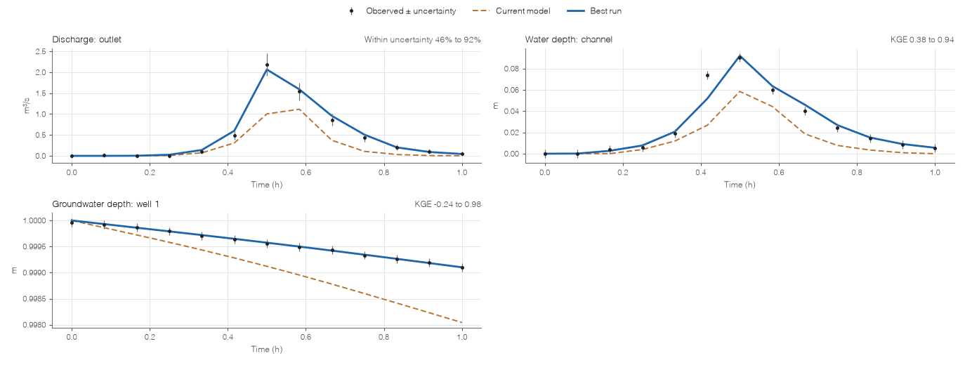
Figure 1. A short calibration in Studio on the twin catchment, with uncertainty on the observations. Discharge is scored with error / uncertainty: 46 % of the points were within their measurement error with the current model, 92 % after calibration.

6.1 GA and SCE-UA

The same twin catchment, with 5 % noise and a budget of about 100 runs per free parameter (Auto, up to 5 runs at a time):

Free parameters	Method	Runs	Best score	Time	Found / true
2	GA	140	0.0089	4.3 min	Manning 1.007, conductivity 1.004
2	SCE-UA	202	0.0074	9.3 min	Manning 1.021, conductivity 1.001
6	GA	481	0.0065	13.9 min	Manning 1.038, conductivity 0.998, specific yield 1.003
6	SCE-UA	659	0.0245	23.8 min	Manning 1.088, conductivity 0.949, specific yield 0.946

With 6 free parameters, the other three were soil α (true × 1.3), soil depth (× 0.8) and groundwater conductivity (× 2). Neither method pinned them down, because these observations say little about them.

• With 2 parameters both recovered the truth. SCE-UA reached a slightly better score, but its 2 complexes let only 2 runs go at once, so it took twice as long.
• With 6 parameters and a few hundred runs, the GA got much further. SCE-UA starts with 78 points and spends 78 to 234 runs per shuffle, so its budget covered only five shuffles.
• SCE-UA pays off with budgets of thousands of runs, as on the test function of Section 4.1. For an expensive model and a few hundred runs, the GA is the default.

A twin experiment is not a field test. It shows that these observations can identify these parameters in this model structure; real records add measurement error, regulation and processes the model leaves out.

---

7. Current Limits

• Point observations (depths, levels, wells) are not recorded on Voronoi and quadtree meshes yet.
• Soil moisture cannot be calibrated yet: its table is shown, but the model reports layer storage, not water content.
• Times are minutes from the start of the run; calendar dates are not read.
• Flood-extent maps are not a target type.
• Studio calibrates one event. The calibration engine also takes several events and validation events, which run only for the best candidate.
• The score is one weighted sum; a Pareto front between kinds of observation is not available.

---

Sources

• Duan, Q., Sorooshian, S., and Gupta, V. (1992). Effective and efficient global optimization for conceptual rainfall-runoff models. Water Resources Research, 28(4), 1015–1031. doi:10.1029/91WR02985
• Duan, Q. Y., Gupta, V. K., and Sorooshian, S. (1993). Shuffled complex evolution approach for effective and efficient global minimization. Journal of Optimization Theory and Applications, 76(3), 501–521. doi:10.1007/BF00939380
• Duan, Q., Sorooshian, S., and Gupta, V. K. (1994). Optimal use of the SCE-UA global optimization method for calibrating watershed models. Journal of Hydrology, 158(3–4), 265–284. doi:10.1016/0022-1694(94)90057-4
• Gupta, H. V., Kling, H., Yilmaz, K. K., and Martinez, G. F. (2009). Decomposition of the mean squared error and NSE performance criteria: implications for improving hydrological modelling. Journal of Hydrology, 377(1–2), 80–91. doi:10.1016/j.jhydrol.2009.08.003
• McKay, M. D., Beckman, R. J., and Conover, W. J. (1979). A comparison of three methods for selecting values of input variables in the analysis of output from a computer code. Technometrics, 21(2), 239–245. doi:10.2307/1268522
• Nash, J. E., and Sutcliffe, J. V. (1970). River flow forecasting through conceptual models, part I: a discussion of principles. Journal of Hydrology, 10(3), 282–290. doi:10.1016/0022-1694(70)90255-6