Groundwater Recession Calibration

HydroPol2D estimates effective, catchment-scale groundwater parameters by matching the simulated outlet recession to an observed master recession curve (MRC). The calibration runs in HydroPol2D-Python. Its accepted results are ordinary case inputs, so Python and MATLAB start from the same parameters and states (see the Model-building workflow).

What the calibration fits depends on the subsurface scheme:

Scheme	Fitted parameters
Default	Uniform horizontal conductivity $K_{sat,h}$ and specific yield $S_y$
Layered	Two multipliers on the horizontal conductivity: one for the soil slots, one for the regolith slots

The fitted values are effective parameters. They reproduce the observed recession under this model structure. They are not point measurements of aquifer material.

The recession calibration is not in HydroPol2D Studio yet. To fit groundwater parameters to well levels or to the discharge of an event, use the calibration against observations (the Calibrate workspace in Studio). Its groundwater-depth series and its conductivity, specific-yield and layered-subsurface multipliers cover that case.

---

1. Workflow

Both schemes use the same steps:

1. Read a local daily-discharge CSV, or download daily discharge from a USGS gauge.
2. Separate baseflow with the Lyne–Hollick filter and assemble the recession events into an MRC.
3. Separate the slow deep-aquifer tail from the faster shallow target.
4. For every candidate, spin the model up to a steady state under the target flow (Section 4).
5. Equilibrate the river state and route the groundwater release through the surface hydraulic solver to the outlet.
6. Score the routed outlet recession against the shallow part of the MRC.
7. Save the best complete hydraulic checkpoint: surface water, shallow groundwater, soil water, deep-aquifer stores and D8 momentum.

The score combines shape and volume, so that high flows do not dominate:

$$J = \mathrm{RMSE}\left(\ln Q_{\mathrm{sim}},\ \ln Q_{\mathrm{obs}}\right) + 0.5\,\frac{\left|V_{\mathrm{sim}} - V_{\mathrm{obs}}\right|}{V_{\mathrm{obs}}}$$

where $V$ is the recession volume over the scored period.

Default scheme:

hydropol2d calibrate-groundwater-recession case.yaml master_recession calibration \
  --usgs-site 02147020 --start-date 1980-01-01 --end-date 2019-09-29 \
  --ksat-values 1e-5,5e-5,1e-4 --specific-yield-values 0.03,0.05,0.1 \
  --shallow-checkpoint-fraction 0.05

For a local file, replace the USGS arguments with --discharge-csv observations.csv. The default columns are date and observed_discharge_m3_s.

---

2. Layered Scheme: Two Lateral-Conductivity Multipliers

With vertical.subsurface.scheme: layered, $S_y$ is not fitted. Each slot takes $S_y$ from its retention curve ($\theta_s - \theta_{fc}$), and a recession constrains only the ratio $K/S_y$ (Brutsaert and Nieber, 1977). The calibration instead fits two catchment-scale factors on the mapped horizontal conductivity:

Parameter	Scales
vertical.subsurface.soil_lateral_conductivity_multiplier	The three soil slots: soil $K_{sat}$ × soil_lateral_anisotropy
vertical.subsurface.regolith_lateral_conductivity_multiplier	The regolith slots: regolith $K_h$ (scalar, raster, or the groundwater $K_{sat}$)

Why two factors can be separated. Early, high flows drain while the water table is in the soil. Late, low flows drain while it is in the regolith. The shape of the recession can therefore separate the two factors. Whether it does depends on the catchment and the record: regulation, noise, and how often the table reaches the soil. Each run reports this (Section 3).

hydropol2d calibrate-groundwater-recession case.yaml master_recession calibration \
  --discharge-csv observations.csv --soil-multipliers 0.1,0.3,1,3,10 \
  --regolith-multipliers 0.1,0.3,1,3,10

---

3. Identifiability Outputs

Every layered run writes coupled_identifiability.json and coupled_objective_surface.png.

Output	Meaning
Acceptable set	Candidates with $J \le 1.05\,J_{\mathrm{best}} + 0.01$
Decades spanned	Range of each multiplier over the acceptable set, in $\log_{10}$ units
Grid-edge flag	Whether the best value sits on the edge of the candidate grid; if so, extend the grid
Log-multiplier correlation	Correlation of the two log multipliers over the acceptable set; strongly negative means a trade-off valley
Recession exponent $b$	Exponent of $-\mathrm{d}Q/\mathrm{d}t = a\,Q^b$, for the target and for each candidate

Both schemes also write:

File	Content
master_recession_curve.csv	Total, shallow and deep observed recession components
coupled_candidate_scores.csv	Objective and diagnostics for every candidate
coupled_best_recession.csv	Observed target and routed outlet recession
coupled_recession_checkpoint.npz	Complete selected initial hydraulic state
coupled_calibration_metadata.json	Parameters, method and checkpoint criterion

The selected checkpoint can be rebased to model time zero. Rebasing keeps the physical water and hydraulic memories and resets the cumulative diagnostics and the mass-balance datum.

---

4. Spin-Up

Each candidate starts from its own steady state under the target flow. This is the main numerical lesson of the layered calibration.

1. Run the model's own column fluxes. The spin-up uses recharge down through the unsaturated slots, the Darcy flux at the table, riverbed drainage every step, and lateral flow on its own clock. The recession therefore does not start with an unsaturated zone that is far from steady.
2. Use 1-h steps first. They run until the window-mean source and the storage range stay within their tolerances over one simulated year.
3. Then use the model's own steps for 30 days.
4. Test steadiness on the storage range, never on end points. A transient that fills fast and drains slowly passes an end-point test at its storage peak.

What went wrong before the fix. In the twin truth run, the soil was left at field capacity at the start of the recession. Capillary rise into that soil reached 0.10 m³/s, against an outflow of 0.005 m³/s. About 50,000 m³ moved into the unsaturated zone in 6 days, and by day 18 the stream was nearly disconnected. Capillary rise, not the aquifer, dominated the recession.

---

5. Twin Experiments

A twin experiment tests identifiability before real data are used:

1. Choose known "true" multipliers.
2. Run the model to make a synthetic recession.
3. Add log-normal noise.
4. Calibrate on the noisy recession.
5. Check whether the truth is recovered.

The tools are in hydropol2d.calibration.recession_twin (run_recession_twin_experiment, write_recession_twin_report).

5.1 Result on a fast-draining valley

This run (2026-10-20) uses the current physics, including the capillary refill rule of the layered subsurface.

Setting	Value
Valley	V-shaped, 11 × 15 cells at 20 m
Specific yield	soil about 0.12, regolith 0.05
Start	1.5 mm/day of outflow
Candidate grid	soil 1, 3, 10 × regolith 0.1, 0.3, 1 (3 × 3)
Truth	soil 3, regolith 0.3
Recession	30 days

Noise	Best candidate	Acceptable candidates	Objective, best	Objective, next best
0 %	soil 3, regolith 0.3	1	0.033	0.123
5 %	soil 3, regolith 0.3	1	0.065	0.117
10 %	soil 3, regolith 0.3	1	0.106	0.131

The truth was recovered at all three noise levels, and it was the only acceptable pair at every level. The nine routed candidates took 68 min on a laptop with 2 workers. All three rows score the same nine routed candidates; only the noise added to the target differs.

In the first run, before the capillary refill rule (2026-10-19), the truth was also the best candidate, but at 10 % noise the soil multiplier was accepted anywhere from 3 to 10.

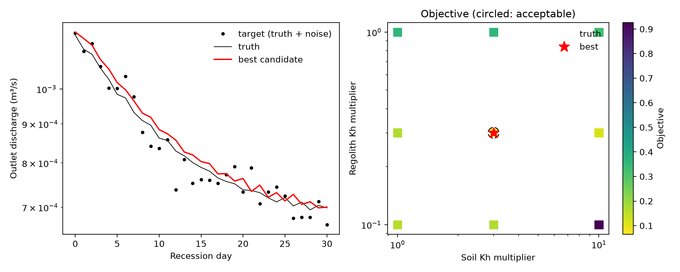
Figure 1. Twin experiment with 5 % noise. Left: target, truth and best candidate. Right: objective over the candidate grid; the circled candidate is the only acceptable one, and it is the truth.

5.2 What limits the test

• Rerun noise. In the 2026-10-19 run, rerunning the same parameters gave a day-to-day spread of ±2.7 %, from a two-interval wobble in the small channel. Differences between candidates below about this size are within run-to-run noise.
• The default twin valley is too slow. With 500 m hillslopes and soil $S_y$ about 0.29, it drains over years. Its recession fell by only 9 % in 20 days, too flat to separate the candidates. For recessions of weeks, use shorter hillslopes and a lower $S_y$, as in Section 5.1.
• A twin test is not a field test. It shows that the method can recover parameters on a synthetic valley with the same model structure. Real records add regulation, evapotranspiration and measurement error.

---

6. Deep-Aquifer Starting State

The same filter, MRC and deep-tail separation give the starting outflow of the deep aquifer:

hydropol2d estimate-deep-baseflow observations.csv --start-date 2019-06-01 \
  --drainage-area-km2 5320 --output deep_baseflow.json

The tool places the start-date baseflow on the MRC and divides its deep part by the drainage area. The report also gives the tail response time, which can be used for deep_aquifer_response_time_days. Pick a start date in a recession: the tool warns when the start-date discharge is more than twice the baseflow. The theory is in Groundwater Model, Section 13.3.

---

7. Case Builder

The Case Builder launches the calibration for either scheme:

1. In a layered case, the launch passes --soil-multipliers and --regolith-multipliers.
2. Finalization writes the fitted multipliers to the Python case (vertical.subsurface) and to the MATLAB runner (HYDROPOL_SOIL_LATERAL_CONDUCTIVITY_MULTIPLIER, HYDROPOL_REGOLITH_LATERAL_CONDUCTIVITY_MULTIPLIER).
3. $S_y$ stays on the retention curves; no uniform $K_{sat}$ or $S_y$ rasters are written.
4. The calibration's DeepAquiferInitialState.json replaces any starting baseflow or mean recharge given by hand.

---

Sources

• Brutsaert, W., and Nieber, J. L. (1977). Regionalized drought flow hydrographs from a mature glaciated plateau. Water Resources Research, 13(3), 637–643. doi:10.1029/WR013i003p00637
• Lyne, V., and Hollick, M. (1979). Stochastic time-variable rainfall-runoff modelling. Institute of Engineers Australia National Conference, Publication 79/10, 89–93.