Groundwater and Recharge Validation

The groundwater section of the validation suite tests both local groundwater bookkeeping and lateral groundwater dynamics. The central implementation change is the asynchronous scheduler: vadose drainage, recharge production, and capillary rise are evaluated every surface-model step, while saturated groundwater storage and lateral heads are updated only when the groundwater scheduler is due.

What was tested

Four V-tilted groundwater cases were used for local storage and scheduler behavior:

• VAL-GW-ASYNC-001: constant recharge water-table rise;
• VAL-GW-ASYNC-002: asynchronous scheduler equivalence;
• VAL-GW-CAP-001: capillary rise drawdown;
• VAL-GW-MOUND-001: Boussinesq recharge mound against a fine-timestep numerical reference.

Two additional hillslope cases were used to strengthen the lateral-groundwater evidence:

• VAL-GW-HILL-STEADY-001: steady Dupuit profile;
• VAL-GW-HILL-TRANSIENT-001: transient linearized Boussinesq decay.

Local recharge and scheduler behavior

Reference and method

The local recharge case uses the analytical storage relation Δh = RΔt / S_y when lateral groundwater flow and exfiltration are disabled. The scheduler-equivalence case compares legacy per-step groundwater updating with the asynchronous accumulation scheduler. The capillary-rise case applies a simple physically capped upward flux from shallow groundwater to dry vadose storage. The recharge-mound case activates lateral groundwater flow and compares the asynchronous result with a fine-timestep internal numerical reference.

Main result

All four local groundwater cases passed.

Case	Regime	Head RMSE (m)	Max head error (m)	Storage error (%)	Residual (m³)
VAL-GW-ASYNC-001	Local recharge	0.0	0.0	0.0	1.96 × 10^-11
VAL-GW-ASYNC-002	Scheduler equivalence	1.71 × 10^-13	1.71 × 10^-13	1.67 × 10^-11	1.84 × 10^-10
VAL-GW-CAP-001	Capillary rise	0.0	0.0	0.0	-1.45 × 10^-12
VAL-GW-MOUND-001	Boussinesq mound	1.83 × 10^-8	9.90 × 10^-8	5.23 × 10^-13	3.09 × 10^-11

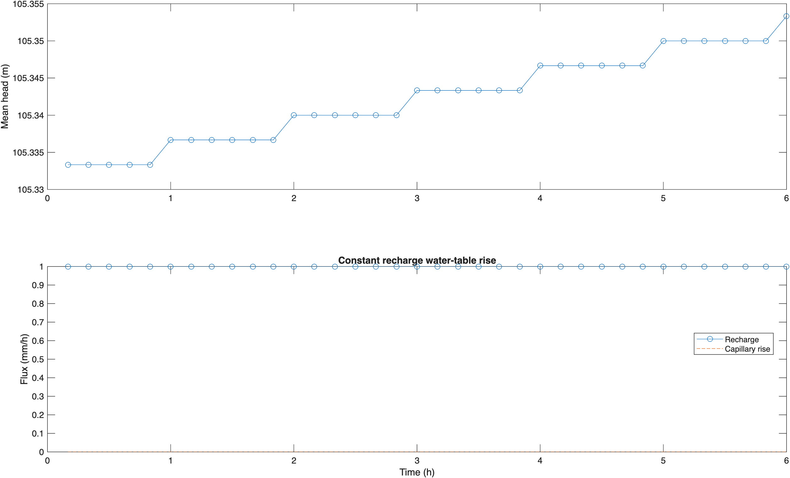
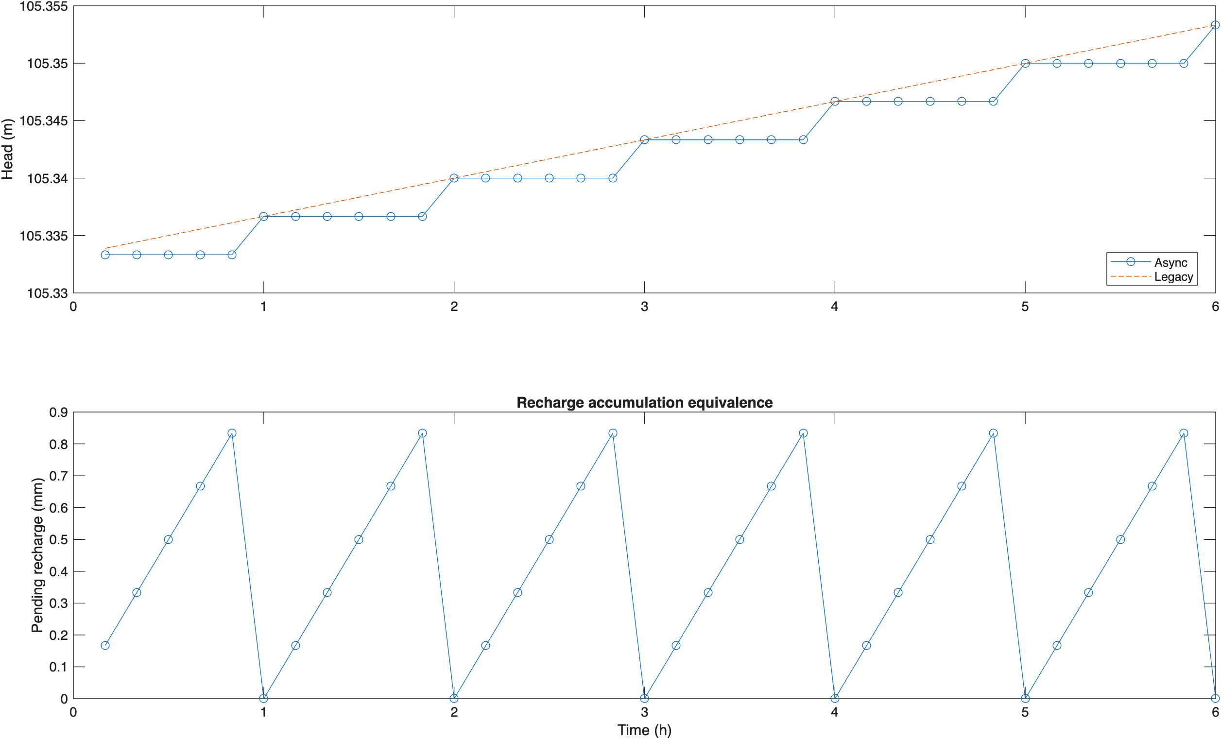
Recharge scheduler diagnostics. The first case checks analytical water-table rise under constant recharge. The second compares the asynchronous scheduler with legacy per-step groundwater updating.

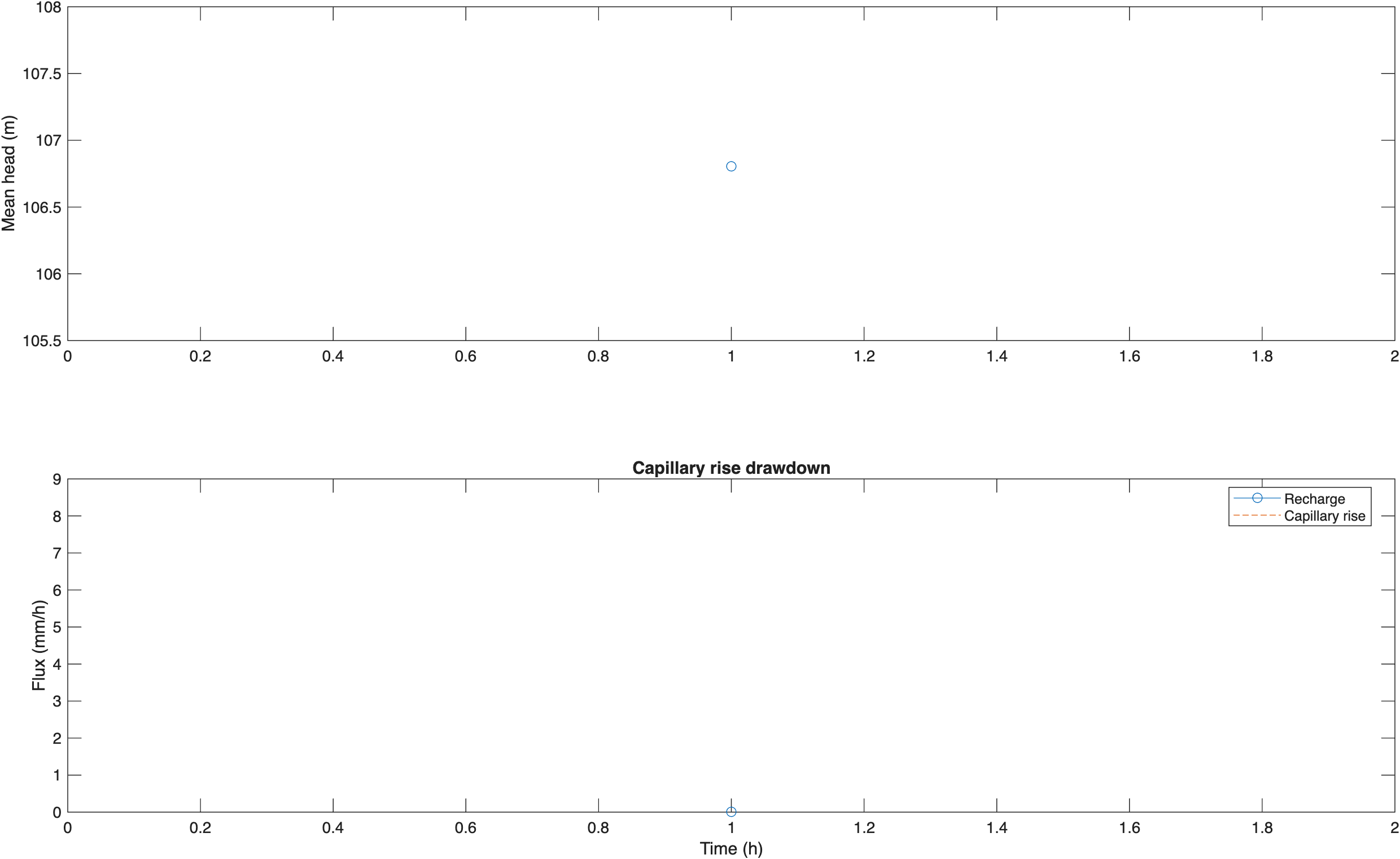
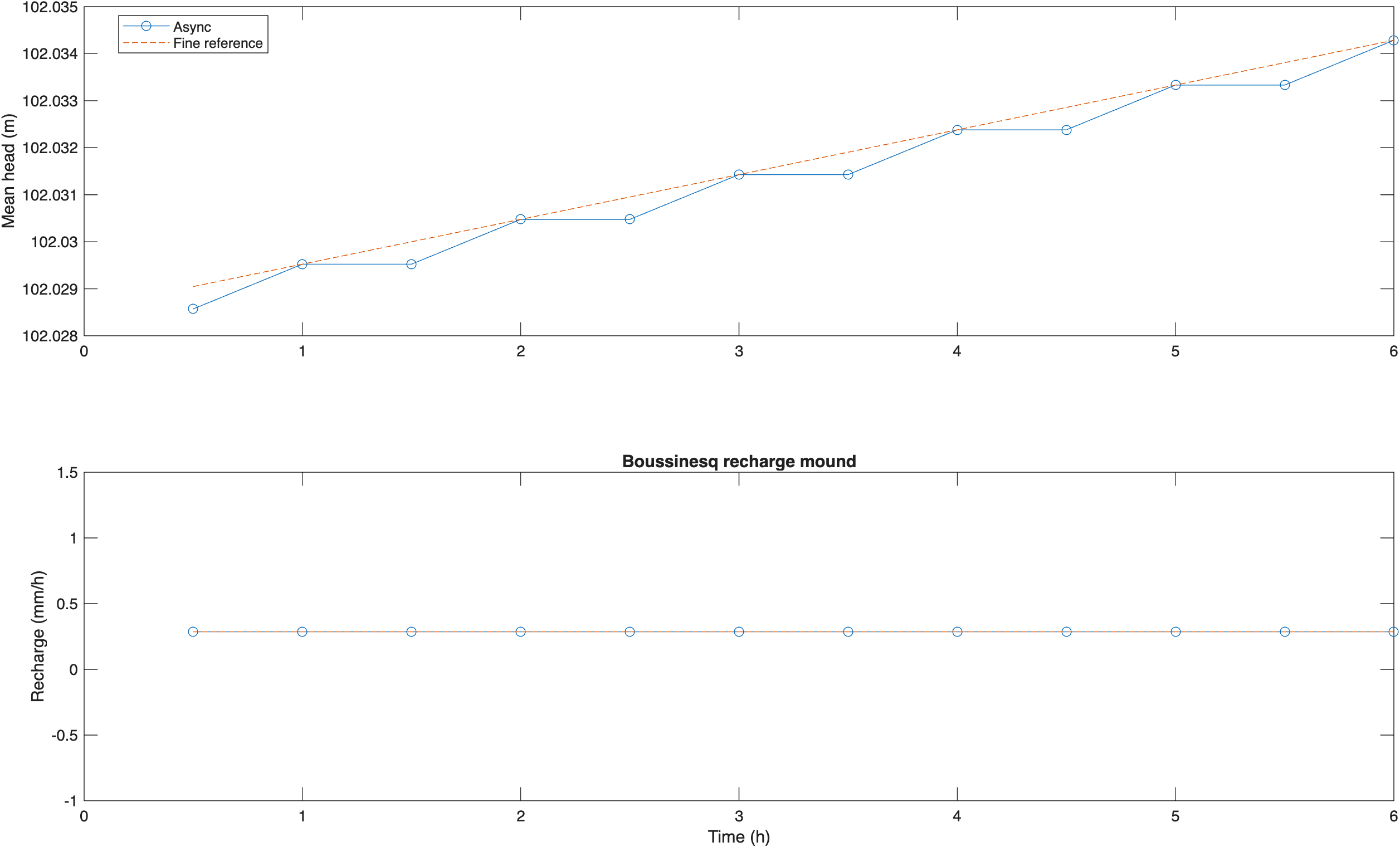
Capillary-rise and lateral-flow diagnostics. The mound case is useful numerical-reference evidence, but it is still weaker than an analytical benchmark.

The main result is that recharge accumulation, asynchronous groundwater updating, and the simple capillary-rise closure all behaved as intended under controlled conditions.

Analytical hillslope benchmarks

Reference and method

The steady hillslope case compares HydroPol2D with the closed-form Dupuit profile under uniform recharge and a fixed drain head. The transient hillslope case compares the HydroPol2D Boussinesq solver with the first eigenmode of the linearized Boussinesq equation in the small-perturbation regime.

Main result

Both analytical hillslope cases passed.

Case	Benchmark	Head RMSE (m)	Max head error (m)	Flow metric
VAL-GW-HILL-STEADY-001	Steady Dupuit	6.04 × 10^-3	9.75 × 10^-3	Drain-discharge error = 3.74 × 10^-4 %
VAL-GW-HILL-TRANSIENT-001	Linearized Boussinesq	1.94 × 10^-5	4.46 × 10^-5	NSE = 0.99985

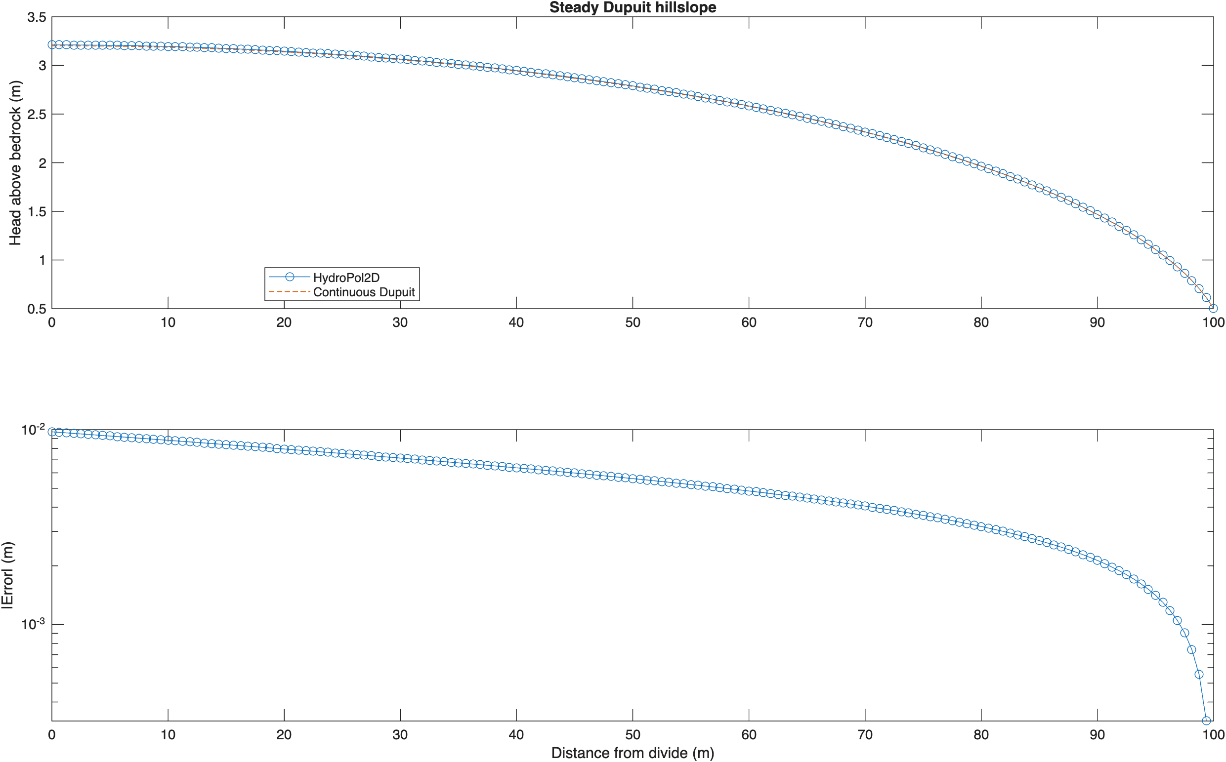
Steady Dupuit benchmark. The lower panel shows the absolute profile error against the analytical solution.

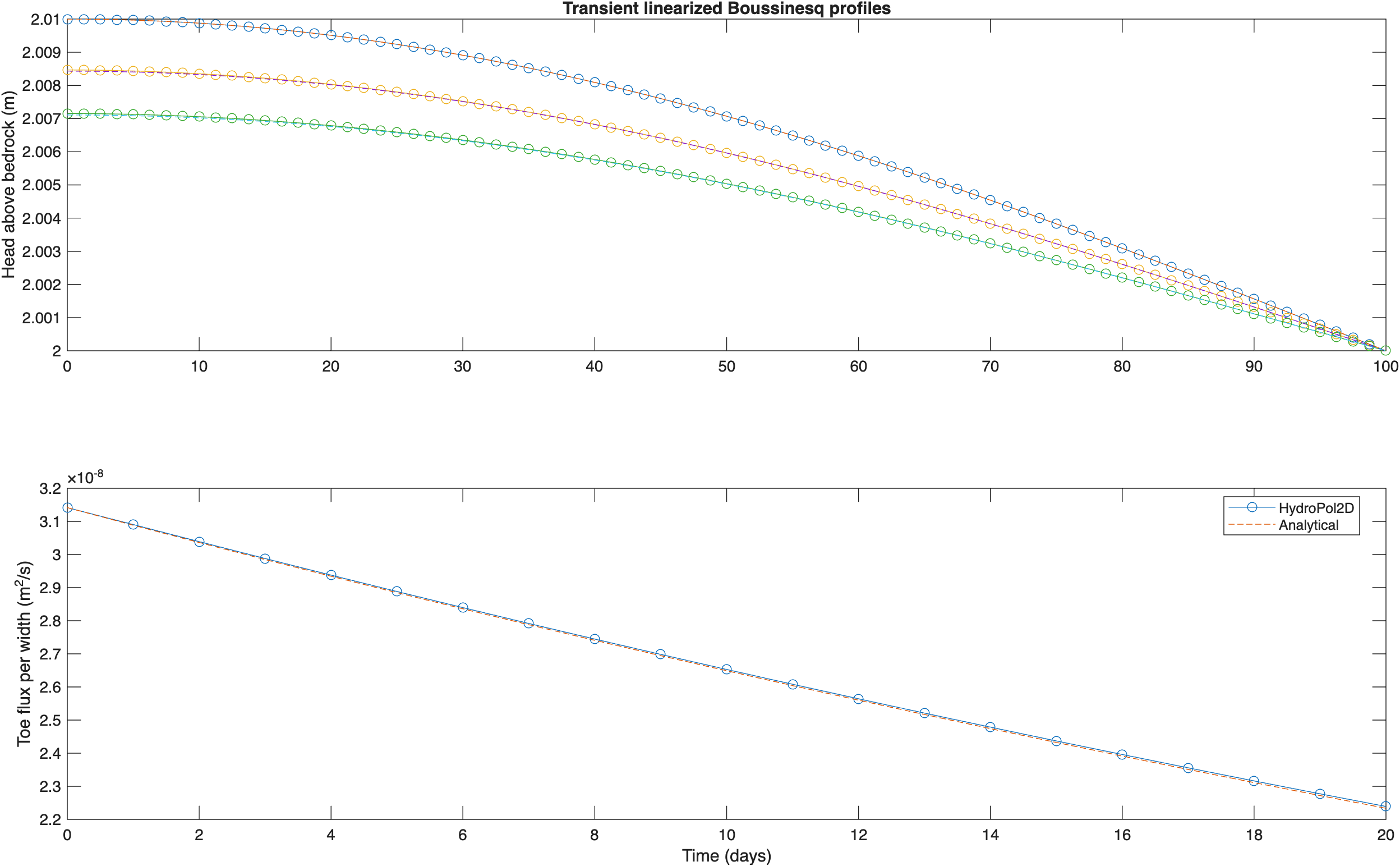
Transient hillslope benchmark. The upper panel compares head profiles during perturbation decay; the lower panel compares modeled and analytical toe flux per unit width.

Layered subsurface

The layered subsurface was added in October 2026. Its evidence is of four kinds: Python unit tests of the column rules, Python-to-MATLAB parity, full-model V-tilted runs in MATLAB, and a calibration twin experiment.

Python column tests

HydroPol2D-Python tests the layered column, Feddes stress and the deep starting state directly (tests/test_subsurface_column.py, test_subsurface_geometry.py, test_subsurface_lateral.py, test_subsurface_mesh.py, test_subsurface_run.py, test_feddes.py, test_deep_aquifer_initial_state.py).

Two numerical tests carry the most weight:

Test	Case	Result
Implicit vs explicit flux	Sand, $\theta = 0.41$, table 30 cm deep (nearly saturated gap), 1-h steps against a 1-s run	Implicit: the table stays within 2 mm of the 1-s run. Explicit: about 20 times too much water drains.
Capillary refill rule	Twin valley, column alone and full model	Water cycling between soil and table 9.3 × 10⁻³ → 0 m³/s; cells flipping sign every step 38 → 0; gross capillary rise 0.016 → 0 m³/s; stream flow unchanged

A further test checks that capillary rise stops at field capacity.

Python-to-MATLAB parity

The MATLAB port is checked against fixtures exported from HydroPol2D-Python (Validation/Groundwater/Layered in the MATLAB repository). Since 2026-10-20 both models have the implicit water-table flux; the kernel fixtures carry implicit and explicit outputs, and the step fixtures use the model default (implicit). MATLAB takes the implicit derivatives by central differences and Python by jax.jvp, so the implicit-flux checks use a tolerance of $10^{-8}$.

Script	What it checks	Recorded result (2026-10-20)
run_layered_kernel_parity.m	Every column kernel: geometry, MMF table update, drainage, Darcy flux (explicit and implicit), Feddes, shared-table bisection, lateral advance	211 checks, worst $2.6 \times 10^{-9}$
run_layered_step_parity.m	The full layered vertical step on a 2 × 2 V-tilted grid, 4 scenarios, 312 steps	3 120 checks, worst $4.9 \times 10^{-11}$
run_layered_vtilted_case.m	Full-model V-tilted runs: local, lateral, feddes, legacy, deep, deep_legacy, deep_empty, and since 2026-10-20 no_dtb (column bottom from the soil table), explicit_flux and soil_rasters	Run from a copy of Examples/VTilted_Excel; lateral volume error $-1.7 \times 10^{-10}$ m³
run_feddes_legacy_consistency.m	Feddes in the default three-layer ET equals layered Feddes ET for the same state; Feddes never takes more than the unstressed rule	consistency check
run_layered_mesh_case.m	20 m V-tilted Voronoi mesh with 2 HRUs: default, layered, layered + Feddes	every step closes mass within $10^{-8}$ of the rain volume

run_deep_aquifer_initial_state_validation.m checks the deep starting state $S_0 = q_0 A \tau$ against a fixture shared with HydroPol2D-Python. Validation/Groundwater/run_groundwater_release_checks.m runs all of these: 17 of 17 passed on 2026-10-20.

Calibration twin experiment

A twin experiment recovered known soil and regolith conductivity multipliers from a synthetic 30-day recession with 0, 5 and 10 % noise; with the capillary refill rule, the truth was the only acceptable pair at every noise level. The setup, results and limits are on the Groundwater Recession Calibration page.

What the layered evidence does not cover

• No field case: the tests use synthetic V-tilted domains.
• The open issues listed under Known Limits, such as perched lateral flow and the missing capillary fringe, are not resolved by these tests.

What this validation supports

Together, these cases support the implemented recharge accumulation, asynchronous scheduler, local water-table rise and drawdown through S_y, simple layered capillary rise, and idealized lateral hillslope groundwater dynamics.

The layered-subsurface tests support the implementation of the soil-over-regolith column and its Python-MATLAB agreement on controlled cases.

They do not validate regional aquifer parameters, field baseflow, groundwater pumping, confined aquifer behavior, or calibration against observed wells.