Case Workbook Settings

A MATLAB case is one workbook, HydroPol2D_Inputs.xlsx. This page lists every setting of its eight settings tabs. The other tabs are described elsewhere:

• class tables (soil, land use, human instability, mesh, control structures): Parameter Tables;
• time series (rain, climate stations, inflow and stage hydrographs): Optional Forcing;
• every switch on one page: Model Flags;
• how to open, fill and run a case: Run from Excel.

Older cases, with General_Data.xlsx, its Flags sheet and separate workbooks, still run. See Older layout.

---

The workbook at a glance

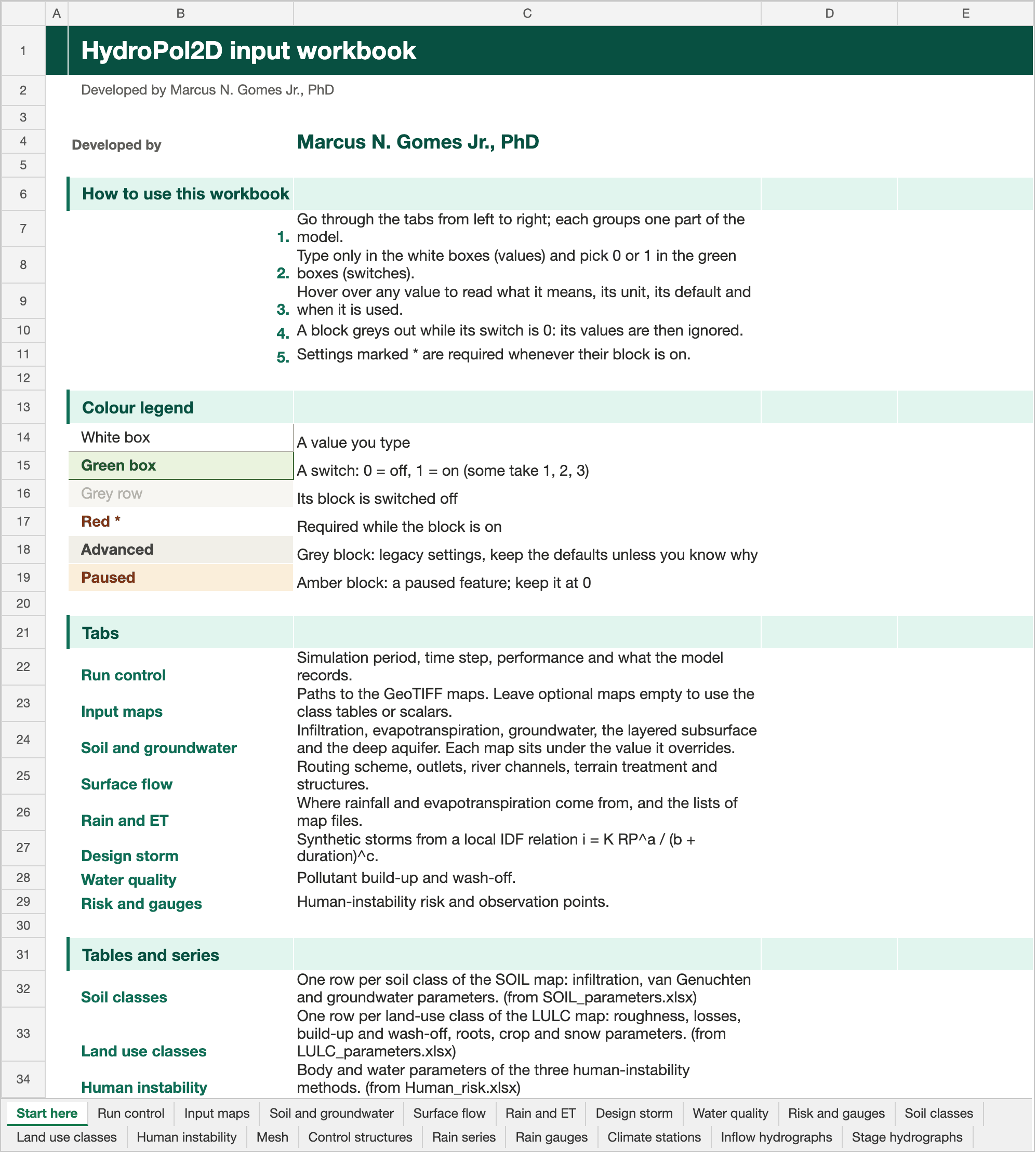
The Start here tab of the Stanford example workbook. Click the picture to open it full size.

Group	Tabs
Guide	Start here: how to fill the workbook, the colour legend and a link to every tab
Settings (8)	Run control, Input maps, Soil and groundwater, Surface flow, Rain and ET, Design storm, Water quality, Risk and gauges
Class tables (5)	Soil classes, Land use classes, Human instability, Mesh, Control structures
Series (5)	Rain series, Rain gauges, Climate stations, Inflow hydrographs, Stage hydrographs

run_HydroPol2D.m reads Input_Data_Sheets/HydroPol2D_Inputs.xlsx by default. HYDROPOL_INPUT_EXCEL_FILE points it to another workbook.

---

How a settings tab works

Each setting is one row: its name, its key, the value, the unit, the default and when it is used. A note on each value explains it.

• Blocks and switches. Settings are grouped in blocks. A block that can be switched off starts with its switch, and its rows grey out while the switch is 0. Greyed values are ignored. There is no separate Flags sheet.
• Required values are marked with a red asterisk. An empty optional value keeps its default or the fallback named in its note.
• Advanced blocks (grey header) hold legacy settings. Keep their defaults unless you know why to change them.
• Paused blocks (amber header) hold paused features. Keep them at 0: setting 1 stops the run.
• Paths can be absolute or relative to the folder of the workbook.

---

Settings reference

The tables below are generated from the catalog that builds the workbook (tools/workbook_builder/input_catalog.yaml in the MATLAB repository), so they match the workbook row for row. The descriptions are the workbook notes.

Run control

Simulation period, time step, performance and what the model records.

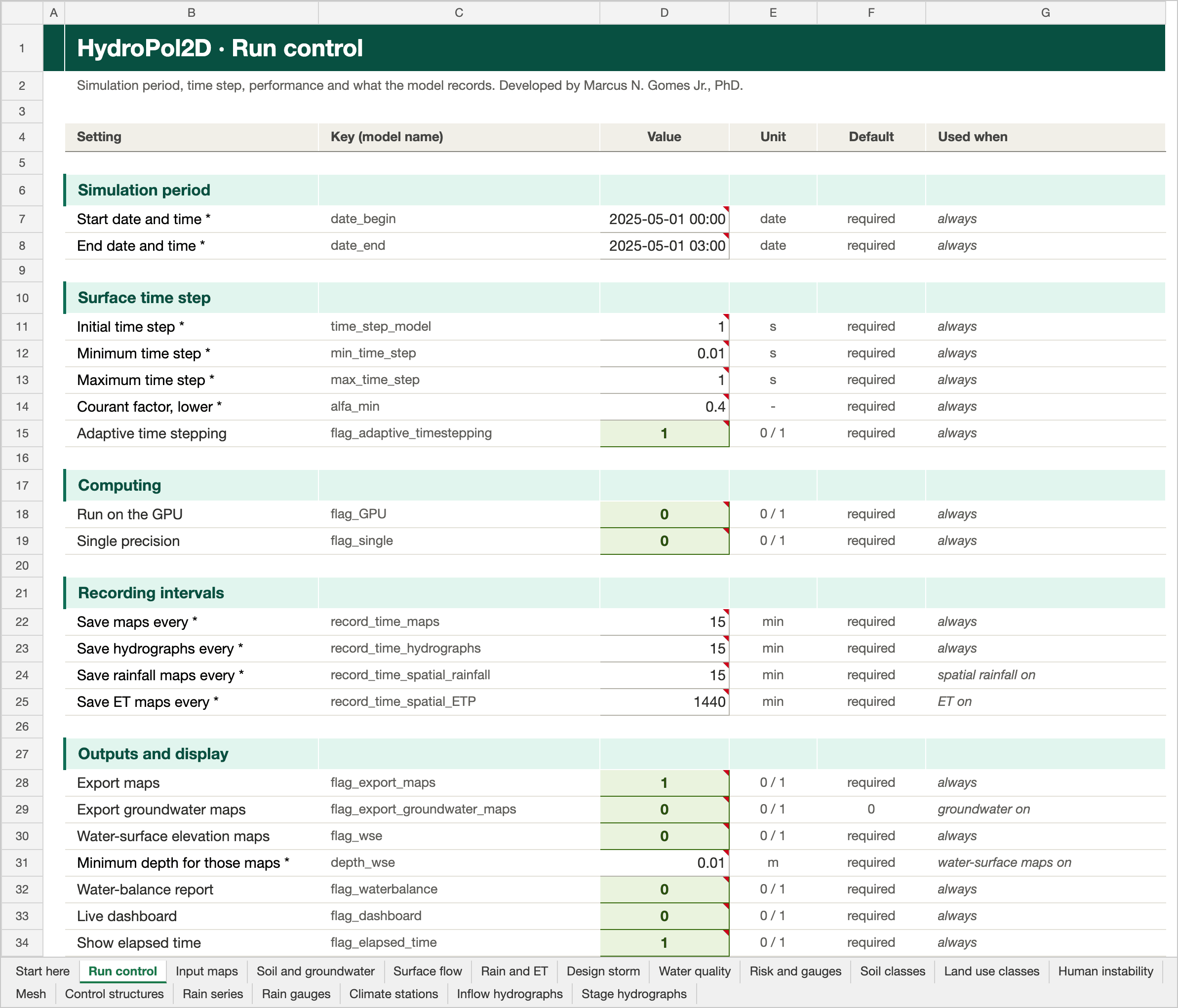
The Run control tab of the Stanford example workbook. Click the picture to open it full size.

Simulation period

Setting	Key	Unit	Default	Used when	Description
Start date and time	date_begin	date	required	always	date_begin is the simulation start datetime. Use the same time reference as rainfall, evapotranspiration, inflow, stage, and observation time series.
End date and time	date_end	date	required	always	date_end is the simulation end datetime. It must be later than date_begin; forcing values outside this interval are not part of the run.

Surface time step

Setting	Key	Unit	Default	Used when	Description
Initial time step	time_step_model	s	required	always	time_step_model is the nominal surface-model timestep in seconds. It initializes the routing loop; adaptive timestepping may replace it with a stable value between min_time_step and max_time_step.
Minimum time step	min_time_step	s	required	always	min_time_step is the smallest allowable surface-routing timestep in seconds. Use a positive value small enough to resolve rapid wetting, shallow flow, and steep terrain.
Maximum time step	max_time_step	s	required	always	max_time_step is the largest allowable surface-routing timestep in seconds. It limits the timestep during slowly varying periods and should be greater than or equal to min_time_step.
Courant factor, lower	alfa_min	-	required	always	alfa_min is the lower Courant safety coefficient used when HydroPol2D calculates a stable surface-routing timestep. Smaller values are more conservative and usually increase runtime.
Adaptive time stepping	flag_adaptive_timestepping	0 / 1	required	always	Updates the surface-routing timestep from the stability limits during the simulation. Keep enabled for most dynamic simulations.

Computing

Setting	Key	Unit	Default	Used when	Description
Run on the GPU	flag_GPU	0 / 1	required	always	Runs supported arrays and calculations on a compatible MATLAB GPU. Leave disabled when a compatible GPU is not available.
Single precision	flag_single	0 / 1	required	always	Stores supported numerical arrays in single precision to reduce memory use. Keep disabled when maximum numerical precision is required.

Recording intervals

Setting	Key	Unit	Default	Used when	Description
Save maps every	record_time_maps	min	required	always	record_time_maps is the interval in minutes between saved spatial model maps. A shorter interval increases output detail and disk use without changing the simulation physics.
Save hydrographs every	record_time_hydrographs	min	required	always	record_time_hydrographs is the interval in minutes between saved outlet, inflow, and gauge hydrograph records. Choose an interval that resolves the expected hydrograph response.
Save rainfall maps every	record_time_spatial_rainfall	min	required	spatial rainfall on	record_time_spatial_rainfall is the interval in minutes used to save or aggregate spatial rainfall information. For raster rainfall, it should be compatible with the map-output interval.
Save ET maps every	record_time_spatial_ETP	min	required	ET on	record_time_spatial_ETP is the interval in minutes between saved spatial evaporation and transpiration products. Shorter intervals produce more detailed files and increase storage demand.

Outputs and display

Setting	Key	Unit	Default	Used when	Description
Export maps	flag_export_maps	0 / 1	required	always	Exports scheduled spatial model outputs such as flood depth and related maps.
Export groundwater maps	flag_export_groundwater_maps	0 / 1	0	groundwater on	Exports scheduled groundwater water-table-depth rasters when groundwater modelling is enabled.
Water-surface elevation maps	flag_wse	0 / 1	required	always	flag_wse controls water-surface-elevation map output: 0 disables it and 1 enables it. The map uses DEM elevation plus simulated water depth where depth exceeds depth_wse.
Minimum depth for those maps	depth_wse	m	required	water-surface maps on	depth_wse is the minimum water depth in metres used when water-surface-elevation maps are produced. It avoids reporting water-surface elevation where the cell is effectively dry.
Water-balance report	flag_waterbalance	0 / 1	required	always	Writes water-balance diagnostics during the run. Enable this for validation and for routine model checks.
Live dashboard	flag_dashboard	0 / 1	required	always	Creates the configured dashboard-oriented outputs during the simulation.
Show elapsed time	flag_elapsed_time	0 / 1	required	always	Prints or records elapsed computational time for the simulation.

Warm start

Setting	Key	Unit	Default	Used when	Description
Start from a warm-up state	flag_warmup	0 / 1	required	always	Initializes the simulation from the configured warm-up state rather than the standard initial-state rasters.

Advanced (keep the defaults unless you know why)

Setting	Key	Unit	Default	Used when	Description
Courant factor, upper	alfa_max	-	required	always	alfa_max is the upper adaptive-timestep coefficient retained for compatible time-control configurations. Keep it positive and no smaller than alfa_min; current routing stability calculations use alfa_min for the conservative candidate step.
Time-step refresh increment	time_step_change	s	required	always	time_step_change is the positive time increment in seconds used for timestep-refresh bookkeeping and diagnostic alignment. It is not the groundwater update interval.
Full time-step stability check	flag_timestep	0 / 1	required	always	Selects the full timestep-stability treatment for supported routing solvers. Use the validated default unless testing a specific numerical formulation.

Input maps

Paths to the GeoTIFF maps. Leave optional maps empty to use the class tables or scalars.

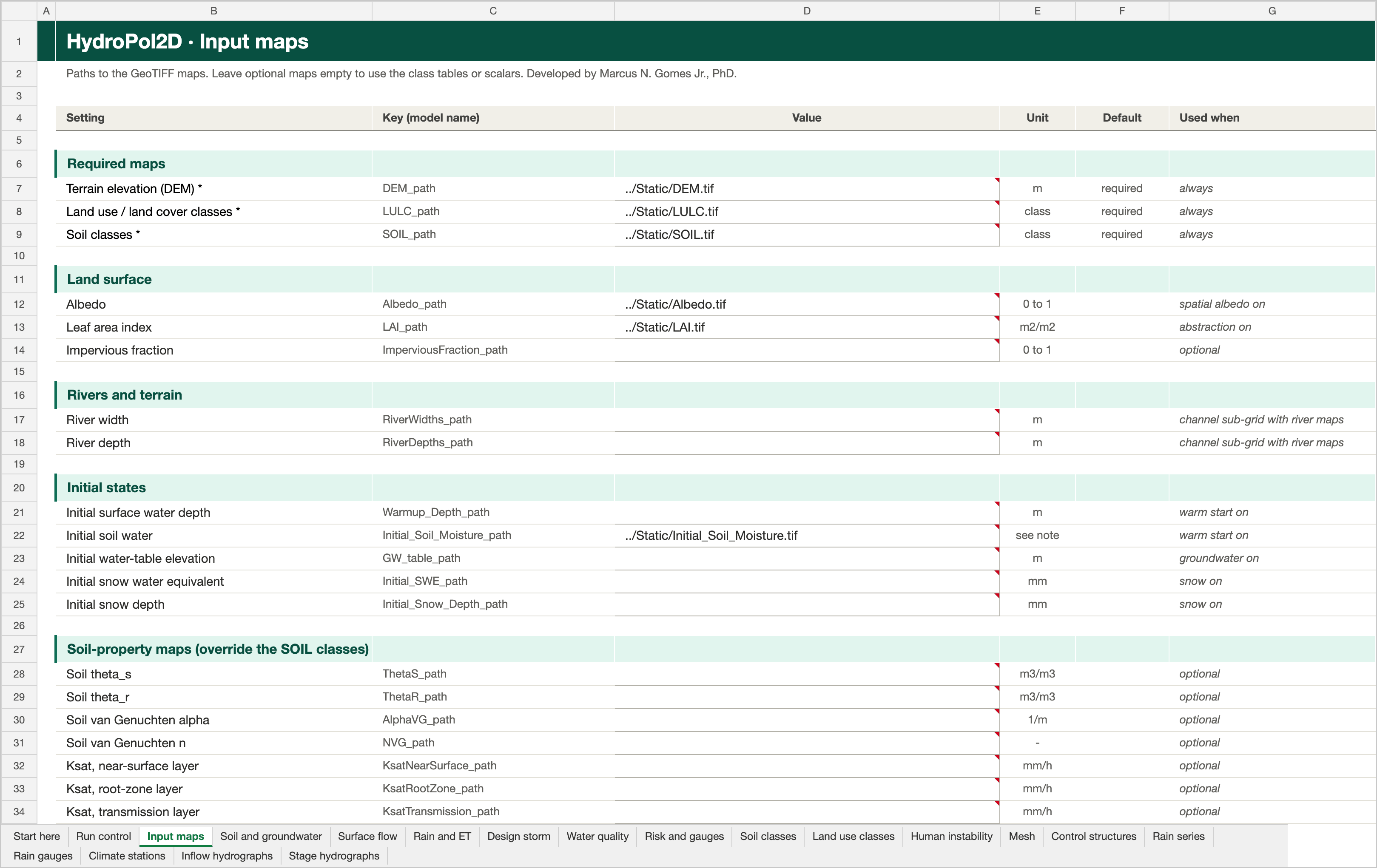
The Input maps tab of the Stanford example workbook. Click the picture to open it full size.

Required maps

Setting	Key	Unit	Default	Used when	Description
Terrain elevation (DEM)	DEM_path	m	required	always	DEM_path is the required path to the terrain elevation GeoTIFF, with elevations in metres. It defines the model domain, grid geometry, and topographic gradients.
Land use / land cover classes	LULC_path	class	required	always	LULC_path is the required categorical land-use/land-cover GeoTIFF. Raster class codes are matched to the Land use classes tab; unmapped codes receive the documented area-weighted fallback.
Soil classes	SOIL_path	class	required	always	SOIL_path is the required categorical soil-class GeoTIFF. Raster class codes are matched to the Soil classes tab; unmapped codes receive the documented area-weighted fallback.

Land surface

Setting	Key	Unit	Default	Used when	Description
Albedo	Albedo_path	0 to 1	empty	spatial albedo on	Albedo_path is an optional raster of surface albedo from 0 to 1. It is used only when spatial albedo is enabled for the energy-balance evapotranspiration calculation.
Leaf area index	LAI_path	m2/m2	empty	abstraction on	LAI_path is an optional leaf-area-index raster in m2 leaf area per m2 ground area. It is used by canopy interception and vegetation-related evapotranspiration when the relevant flags are enabled.
Impervious fraction	ImperviousFraction_path	0 to 1	empty	optional	ImperviousFraction_path is an optional raster of fractional impervious cover from 0 to 1. It refines infiltration behavior within a cell; values outside this range are not physically meaningful.

Rivers and terrain

Setting	Key	Unit	Default	Used when	Description
River width	RiverWidths_path	m	empty	channel sub-grid with river maps	RiverWidths_path is an optional river-width GeoTIFF in metres. It is required for the active Neal (2012) embedded-channel model when flag_subgrid and flag_river_rasters are enabled; valid embedded widths must remain smaller than the coarse-cell size.
River depth	RiverDepths_path	m	empty	channel sub-grid with river maps	RiverDepths_path is an optional river-depth GeoTIFF in metres. It is paired with RiverWidths_path for the active embedded-channel model and must be positive where a channel is present.

Initial states

Setting	Key	Unit	Default	Used when	Description
Initial surface water depth	Warmup_Depth_path	m	empty	warm start on	Warmup_Depth_path is an optional initial surface-water-depth GeoTIFF in metres. It is read only when flag_warmup is enabled and initializes surface storage before routing.
Initial soil water	Initial_Soil_Moisture_path	see note	empty	warm start on	Initial_Soil_Moisture_path is an optional initial soil-water-storage GeoTIFF. Despite its legacy name, values are interpreted as storage above residual moisture in mm, not as volumetric water content; it is read with flag_warmup.
Initial water-table elevation	GW_table_path	m	empty	groundwater on	GW_table_path is an optional initial groundwater-table elevation GeoTIFF in metres, using the same vertical datum as the DEM. It is read when groundwater or baseflow is enabled and is constrained below the land surface.
Initial snow water equivalent	Initial_SWE_path	mm	empty	snow on	Initial_SWE_path is an optional initial snow-water-equivalent GeoTIFF in mm water equivalent. It is read only when snow modeling is enabled; negative values are invalid and no-data cells use the default zero-snow condition.
Initial snow depth	Initial_Snow_Depth_path	mm	empty	snow on	Initial_Snow_Depth_path is an optional initial snow-depth GeoTIFF in mm. It is read only when snow modeling is enabled; when paired with SWE, the model checks their physical consistency and derives density.

Soil-property maps (override the SOIL classes)

Setting	Key	Unit	Default	Used when	Description
Soil theta_s	ThetaS_path	m3/m3	empty	optional	ThetaS_path is an optional GeoTIFF of the soil saturated water content theta_s in m3/m3. It overrides the SOIL_parameters value of each class where finite (nodata keeps the class value), for all soil layers.
Soil theta_r	ThetaR_path	m3/m3	empty	optional	ThetaR_path is an optional GeoTIFF of the soil residual water content theta_r in m3/m3. It overrides the SOIL_parameters value of each class where finite (nodata keeps the class value).
Soil van Genuchten alpha	AlphaVG_path	1/m	empty	optional	AlphaVG_path is an optional GeoTIFF of the soil van Genuchten alpha in 1/m. It overrides the SOIL_parameters value of each class where finite (nodata keeps the class value).
Soil van Genuchten n	NVG_path	-	empty	optional	NVG_path is an optional GeoTIFF of the soil van Genuchten n (greater than 1, dimensionless). It overrides the SOIL_parameters value of each class where finite (nodata keeps the class value).
Ksat, near-surface layer	KsatNearSurface_path	mm/h	empty	optional	KsatNearSurface_path is an optional GeoTIFF of the saturated hydraulic conductivity of the near-surface soil layer in mm/h. It overrides ksat x Ks_multiplier_near_surface of each SOIL class where finite (nodata keeps the class value).
Ksat, root-zone layer	KsatRootZone_path	mm/h	empty	optional	KsatRootZone_path is an optional GeoTIFF of the saturated hydraulic conductivity of the root-zone soil layer in mm/h. It overrides ksat x Ks_multiplier_root_zone of each SOIL class where finite (nodata keeps the class value).
Ksat, transmission layer	KsatTransmission_path	mm/h	empty	optional	KsatTransmission_path is an optional GeoTIFF of the saturated hydraulic conductivity of the transmission soil layer in mm/h. It overrides ksat x Ks_multiplier_transmission of each SOIL class where finite (nodata keeps the class value).
Aquifer Ksat (kgsat)	GroundwaterKsat_path	mm/h	empty	optional	GroundwaterKsat_path is an optional GeoTIFF of the aquifer horizontal conductivity kgsat in mm/h. It overrides the SOIL_parameters kgsat of each class where finite. Layered subsurface: it is the rock Kh fallback when regolith_ksat_h_mm_h and RegolithKsatH_path are empty.
Aquifer specific yield	SpecificYield_path	-	empty	legacy groundwater	SpecificYield_path is an optional GeoTIFF of the aquifer specific yield Sy (dimensionless) for the legacy groundwater scheme. It overrides the SOIL_parameters Sy of each class where finite. Not used by the layered subsurface, where Sy comes from the retention curves (or regolith_specific_yield).

Water-quality maps

Setting	Key	Unit	Default	Used when	Description
Initial pollutant mass	Initial_Buildup_path	kg/cell	empty	initial build-up on	Initial_Buildup_path is an optional pollutant-mass GeoTIFF in kg per cell. It is read only when flag_initial_buildup and the water-quality module are enabled.
Build-up asymptote C1	B1_path	see note	empty	water quality with maps	B1_path is an optional GeoTIFF path for the spatial C1 buildup asymptote. It is read only when water quality and raster water-quality inputs are enabled; use values and units consistent with the LULC C1 parameter.
Build-up rate C2	B2_path	see note	empty	water quality with maps	B2_path is an optional GeoTIFF path for the spatial C2 buildup-rate parameter. It is read only when water quality and raster water-quality inputs are enabled.
Wash-off coefficient C3	W1_path	see note	empty	water quality with maps	W1_path is an optional GeoTIFF path for the spatial C3 washoff coefficient. It is read only when water quality and raster water-quality inputs are enabled.
Wash-off exponent C4	W2_path	see note	empty	water quality with maps	W2_path is an optional GeoTIFF path for the spatial C4 washoff exponent. It is read only when water quality and raster water-quality inputs are enabled.

Soil and groundwater

Infiltration, evapotranspiration, groundwater, the layered subsurface and the deep aquifer. Each map sits under the value it overrides.

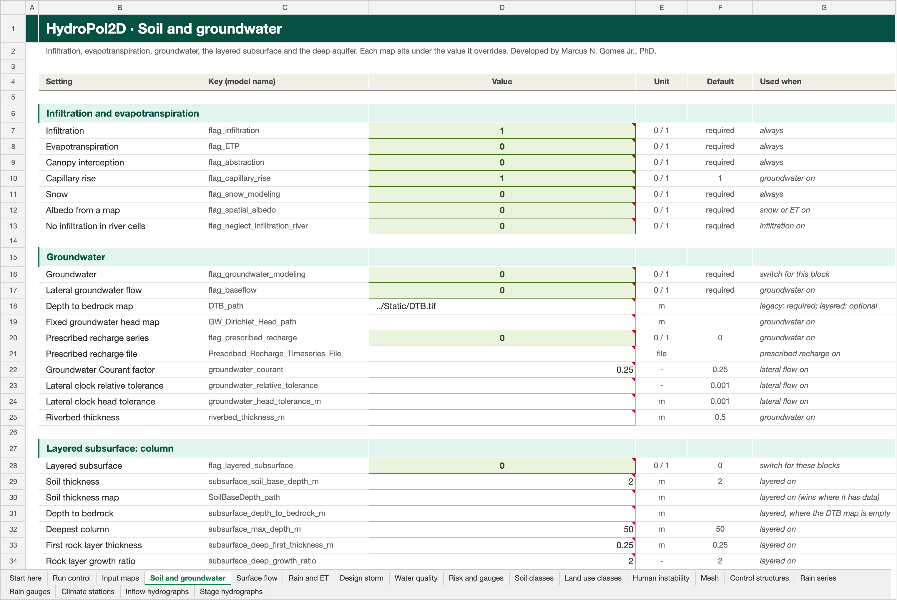
The Soil and groundwater tab of the Stanford example workbook. Click the picture to open it full size.

Infiltration and evapotranspiration

Setting	Key	Unit	Default	Used when	Description
Infiltration	flag_infiltration	0 / 1	required	always	Enables infiltration and the layered soil-water balance. Disabling it also disables evapotranspiration in the current model.
Evapotranspiration	flag_ETP	0 / 1	required	always	Enables evapotranspiration. HydroPol2D uses the configured meteorological or map inputs to calculate evaporation and transpiration.
Canopy interception	flag_abstraction	0 / 1	required	always	Enables canopy interception and initial abstraction processes.
Capillary rise	flag_capillary_rise	0 / 1	1	groundwater on	Enables capped upward flow from shallow groundwater to the transmission or root zone when storage deficits exist.
Snow	flag_snow_modeling	0 / 1	required	always	Enables precipitation partition, snow storage, melt, sublimation, and compaction using the snow columns of the Land use classes tab.
Albedo from a map	flag_spatial_albedo	0 / 1	required	snow or ET on	Uses the supplied albedo raster instead of the scalar default albedo.
No infiltration in river cells	flag_neglect_infiltration_river	0 / 1	required	infiltration on	Sets infiltration and initial abstraction to zero in identified river cells.

Groundwater

Switch: flag_groundwater_modeling. The rest of the block greys out while it is 0.

Setting	Key	Unit	Default	Used when	Description
Groundwater	flag_groundwater_modeling	0 / 1	required	switch for this block	Enables the coupled layered-soil recharge and saturated groundwater module.
Lateral groundwater flow	flag_baseflow	0 / 1	required	groundwater on	Enables the configured baseflow contribution where the selected hydrologic workflow supports it.
Depth to bedrock map	DTB_path	m	empty	legacy: required; layered: optional	DTB_path is an optional DEPTH-TO-BEDROCK GeoTIFF in metres below the land surface. Legacy groundwater: it is the soil depth, and the aquifer lives inside it. Layered subsurface: it is the bottom of the whole column (soil plus weathered rock); the soil thickness is set separately by subsurface_soil_base_depth_m or SoilBaseDepth_path. Required for legacy groundwater; optional with flag_layered_subsurface = 1, where an empty DTB_path falls back to subsurface_depth_to_bedrock_m, then to the DTB (m) of each soil class in the Soil classes tab.
Fixed groundwater head map	GW_Dirichlet_Head_path	m	empty	groundwater on	GW_Dirichlet_Head_path is an optional prescribed groundwater-head elevation GeoTIFF in metres. Finite raster cells define the groundwater Dirichlet boundary; no-data cells remain unconstrained.
Prescribed recharge series	flag_prescribed_recharge	0 / 1	0	groundwater on	Replaces the computed recharge to the water table with the series in Prescribed_Recharge_Timeseries_File (Input maps tab). Default 0.
Prescribed recharge file	Prescribed_Recharge_Timeseries_File	file	empty	prescribed recharge on	Prescribed_Recharge_Timeseries_File is an optional file with a recharge time series that replaces the computed recharge to the water table. It is read only when flag_prescribed_recharge = 1.
Groundwater Courant factor	groundwater_courant	-	0.25	lateral flow on	groundwater_courant is the dimensionless safety factor used to limit the Boussinesq groundwater timestep. Use a value greater than zero and no greater than one; smaller values improve stability at the cost of more updates.
Lateral clock relative tolerance	groundwater_relative_tolerance	-	0.001	lateral flow on	groundwater_relative_tolerance is the relative change of groundwater storage that triggers the next lateral groundwater update (the lateral clock). Smaller values update more often and cost more. Default 0.001.
Lateral clock head tolerance	groundwater_head_tolerance_m	m	0.001	lateral flow on	groundwater_head_tolerance_m is the water-table change in metres that triggers the next lateral groundwater update (the lateral clock). Smaller values update more often and cost more. Default 0.001 m.
Riverbed thickness	riverbed_thickness_m	m	0.5	groundwater on	riverbed_thickness_m is the riverbed thickness in metres used in the river-aquifer exchange: conductance = riverbed Ksat x riverbed area / thickness. Default 0.5 m.

Layered subsurface: column

Switch: flag_layered_subsurface. The rest of the block greys out while it is 0.

Setting	Key	Unit	Default	Used when	Description
Layered subsurface	flag_layered_subsurface	0 / 1	0	switch for these blocks	Enables the layered subsurface: three soil layers over weathered-rock layers down to bedrock, one water table per cell (Miguez-Macho et al., 2007 rules). Settings are in the layered-subsurface blocks of the Soil and groundwater tab; the optional rasters sit under the values they override. Requires flag_groundwater_modeling = 1.
Soil thickness	subsurface_soil_base_depth_m	m	2.0	layered on	subsurface_soil_base_depth_m is the SOIL THICKNESS in metres below ground: where the soil ends and weathered rock (regolith) begins. The three soil layers (near-surface, root zone, transmission) use the Soil classes tab down to this depth. SoilBaseDepth_path overrides it cell by cell. It is capped at the depth to bedrock. Default 2.0 m.
Soil thickness map	SoilBaseDepth_path	m	empty	layered on (wins where it has data)	SoilBaseDepth_path is an optional GeoTIFF of SOIL THICKNESS in metres below ground (the soil base). It overrides subsurface_soil_base_depth_m where finite. Layered subsurface only. Global source: SoilGrids BDRICM.
Depth to bedrock	subsurface_depth_to_bedrock_m	m	empty	layered, where the DTB map is empty	subsurface_depth_to_bedrock_m is the DEPTH TO BEDROCK in metres below ground: the bottom of the whole modelled column, soil plus the weathered rock below it. It is deeper than (or equal to) the soil thickness. Priority: DTB_path raster, then this value, then the DTB (m) of each soil class in the Soil classes tab, with a warning. Capped at subsurface_max_depth_m.
Deepest column	subsurface_max_depth_m	m	50.0	layered on	subsurface_max_depth_m caps the modelled column in metres below ground: column bottom = min(depth to bedrock, this value). Default 50 m.
First rock layer thickness	subsurface_deep_first_thickness_m	m	0.25	layered on	subsurface_deep_first_thickness_m is the thickness in metres of the first rock layer directly below the soil base. Each next layer is subsurface_deep_growth_ratio times thicker, up to subsurface_deep_max_thickness_m. Default 0.25 m.
Rock layer growth ratio	subsurface_deep_growth_ratio	-	2.0	layered on	subsurface_deep_growth_ratio multiplies each rock layer's thickness to get the next one: 0.25, 0.5, 1, 2, 4, 4, ... m with the defaults. Use a value of at least 1. Default 2.
Thickest rock layer	subsurface_deep_max_thickness_m	m	4.0	layered on	subsurface_deep_max_thickness_m is the largest rock-layer thickness in metres. Layers keep this thickness down to the column bottom. Default 4 m.

Layered subsurface: rock properties

Greyed out while flag_layered_subsurface is 0.

Setting	Key	Unit	Default	Used when	Description
Rock theta_s	regolith_theta_s	m3/m3	0.35	layered on	regolith_theta_s is the saturated water content (porosity) of the rock layers below the soil base, in m3/m3. RegolithThetaS_path overrides it cell by cell. Default 0.35.
Rock theta_s map	RegolithThetaS_path	m3/m3	empty	layered on (wins where it has data)	RegolithThetaS_path is an optional GeoTIFF of the rock-layer saturated water content in m3/m3. It overrides regolith_theta_s where finite. Layered subsurface only.
Rock theta_r	regolith_theta_r	m3/m3	0.05	layered on	regolith_theta_r is the residual water content of the rock layers, in m3/m3, below regolith_theta_s. RegolithThetaR_path overrides it cell by cell. Default 0.05.
Rock theta_r map	RegolithThetaR_path	m3/m3	empty	layered on (wins where it has data)	RegolithThetaR_path is an optional GeoTIFF of the rock-layer residual water content in m3/m3. It overrides regolith_theta_r where finite. Layered subsurface only.
Rock van Genuchten alpha	regolith_alpha_vg_m_inverse	1/m	2.0	layered on	regolith_alpha_vg_m_inverse is the van Genuchten alpha of the rock layers, in 1/m. With regolith_n_vg it sets how much water the rock keeps after draining, and so its specific yield. RegolithAlphaVG_path overrides it cell by cell. Default 2.
Rock van Genuchten alpha map	RegolithAlphaVG_path	1/m	empty	layered on (wins where it has data)	RegolithAlphaVG_path is an optional GeoTIFF of the rock-layer van Genuchten alpha in 1/m. It overrides regolith_alpha_vg_m_inverse where finite. Layered subsurface only.
Rock van Genuchten n	regolith_n_vg	-	1.5	layered on	regolith_n_vg is the van Genuchten n of the rock layers (dimensionless, greater than 1). RegolithNVG_path overrides it cell by cell. Default 1.5.
Rock van Genuchten n map	RegolithNVG_path	-	empty	layered on (wins where it has data)	RegolithNVG_path is an optional GeoTIFF of the rock-layer van Genuchten n. It overrides regolith_n_vg where finite. Layered subsurface only.
Rock vertical Ksat	regolith_ksat_v_mm_h	mm/h	5.0	layered on	regolith_ksat_v_mm_h is the vertical saturated hydraulic conductivity of the rock layers in mm/h. It limits drainage and recharge through the rock. RegolithKsatV_path overrides it cell by cell. Default 5 mm/h.
Rock vertical Ksat map	RegolithKsatV_path	mm/h	empty	layered on (wins where it has data)	RegolithKsatV_path is an optional GeoTIFF of the rock-layer vertical saturated conductivity in mm/h. It overrides regolith_ksat_v_mm_h where finite. Layered subsurface only.
Rock horizontal Ksat	regolith_ksat_h_mm_h	mm/h	empty	layered on (empty: kgsat)	regolith_ksat_h_mm_h is the horizontal saturated hydraulic conductivity of the rock layers in mm/h, used for lateral groundwater flow. Leave it empty to use the groundwater Ksat (kgsat) of the Soil classes tab. RegolithKsatH_path overrides it cell by cell.
Rock horizontal Ksat map	RegolithKsatH_path	mm/h	empty	layered on (wins where it has data)	RegolithKsatH_path is an optional GeoTIFF of the rock-layer horizontal saturated conductivity in mm/h, used for lateral groundwater flow. It overrides regolith_ksat_h_mm_h where finite. Layered subsurface only. Global source: GLHYMPS 2.0 permeability.
Rock specific yield	regolith_specific_yield	-	empty	layered on (empty: from curve)	regolith_specific_yield is the drainable porosity of the rock layers (dimensionless). Leave it empty to derive it from the van Genuchten values as theta_s minus the water content at field capacity. A value here or RegolithSpecificYield_path overrides that; it must not exceed theta_s minus theta_r.
Rock specific yield map	RegolithSpecificYield_path	-	empty	layered on (wins where it has data)	RegolithSpecificYield_path is an optional GeoTIFF of the rock-layer specific yield. It overrides the derived value (theta_s minus field capacity) where finite. Layered subsurface only.

Layered subsurface: soil and numerics

Greyed out while flag_layered_subsurface is 0.

Setting	Key	Unit	Default	Used when	Description
Soil Kh / Kv	soil_lateral_anisotropy	-	1.0	layered on	soil_lateral_anisotropy is the horizontal-to-vertical conductivity ratio of the three soil layers: Kh = anisotropy x Ksat. 1 means isotropic. Default 1.
Field-capacity suction	capillary_field_capacity_head_m	m	3.3	layered on	capillary_field_capacity_head_m is the suction head in metres that defines field capacity: the water a layer keeps after the water table falls out of it. Specific yield = theta_s minus theta at this head, and capillary rise from the water table refills a layer only up to this water content. Default 3.3 m (about 33 kPa). Lower it to represent a capillary fringe above shallow water tables (specific yield falls with it).
Drainage sub-steps	subsurface_drainage_substeps	-	1	layered on	subsurface_drainage_substeps is the number of sub-steps for gravity drainage between layers inside one model timestep. 1 is enough for most cases; raise it (2 to 10) for thin, highly conductive layers. Default 1.
Lateral update interval	groundwater_target_dt_s	s	86400	groundwater on	groundwater_target_dt_s is the interval in seconds between lateral groundwater updates, in both subsurface schemes. A shorter interval is used when the stability limit requires it. Vertical soil fluxes still run every model timestep. Default 86400 s (one day).
Shortest lateral interval	groundwater_min_dt_s	s	60	groundwater on	groundwater_min_dt_s is the shortest interval in seconds allowed between lateral groundwater updates, even when the stability limit asks for less. Default 60 s.
Implicit water-table flux	flag_implicit_water_table_flux	0 / 1	1	layered on	Solves the Darcy flux between the soil and the water table implicitly in the layered subsurface (one linearised backward-Euler step per cell): 1 (default) stays accurate at long time steps when the water table is shallow; 0 uses the explicit flux, which needs short steps there. Used only with flag_layered_subsurface = 1.

Lateral conductivity multipliers

Greyed out while flag_layered_subsurface is 0.

Setting	Key	Unit	Default	Used when	Description
Soil Kh multiplier	soil_lateral_conductivity_multiplier	-	1.0	layered on	soil_lateral_conductivity_multiplier scales the horizontal conductivity of the three soil layers (soil Ksat x soil_lateral_anisotropy) for lateral groundwater flow. Vertical Ksat and infiltration do not change. Fitted by the layered groundwater recession calibration (high flows drain through the soil); 1 keeps the mapped values.
Rock Kh multiplier	regolith_lateral_conductivity_multiplier	-	1.0	layered on	regolith_lateral_conductivity_multiplier scales the horizontal conductivity of the rock layers below the soil base (regolith_ksat_h_mm_h, RegolithKsatH_path or kgsat). Fitted by the layered groundwater recession calibration (low flows drain through the rock); 1 keeps the mapped values.

Feddes root-water stress

Switch: flag_feddes. The rest of the block greys out while it is 0.

Setting	Key	Unit	Default	Used when	Description
Feddes stress	flag_feddes	0 / 1	0	switch for this block	Enables Feddes root-water stress: transpiration from each soil layer is reduced by its suction head. Heads are in this block. Works with the layered and the legacy soil schemes.
h1, anaerobiosis	feddes_h1_m	m	-0.1	Feddes on	feddes_h1_m is the anaerobiosis head in metres (negative). Wetter than h1, roots take no water (no oxygen). Default -0.1 m.
h2, optimal from	feddes_h2_m	m	-0.25	Feddes on	feddes_h2_m is the head in metres (negative) where uptake becomes optimal. Between h1 and h2 the stress factor rises from 0 to 1. Default -0.25 m.
h3, stress from	feddes_h3_m	m	-4.0	Feddes on	feddes_h3_m is the head in metres (negative) where water stress starts. Between h3 and h4 the factor falls from 1 to 0. Used when feddes_h3_low_m and feddes_h3_high_m are empty. Default -4 m.
h3 at low demand	feddes_h3_low_m	m	empty	Feddes on (empty: h3)	feddes_h3_low_m is h3 at low transpiration demand (potential ET of 1 mm/d or less), in metres (negative). With feddes_h3_high_m, h3 is interpolated by demand as in SWAP. Leave it empty to use feddes_h3_m.
h3 at high demand	feddes_h3_high_m	m	empty	Feddes on (empty: h3)	feddes_h3_high_m is h3 at high transpiration demand (potential ET of 5 mm/d or more), in metres (negative); usually less negative than feddes_h3_low_m, so stress starts earlier on high-demand days. Leave it empty to use feddes_h3_m.
h4, wilting point	feddes_h4_m	m	-80.0	Feddes on	feddes_h4_m is the wilting-point head in metres (negative). Drier than h4, roots take no water. Default -80 m (-0.8 MPa).

Deep aquifer

Switch: flag_deep_aquifer. The rest of the block greys out while it is 0.

Setting	Key	Unit	Default	Used when	Description
Deep aquifer	flag_deep_aquifer	0 / 1	0	switch for this block	Enables the deep aquifer: deep_recharge_fraction of the water-table recharge goes to one linear reservoir per subbasin and returns to the surface after deep_aquifer_tau_days. Requires DeepAquiferSubbasins_path and DeepAquiferChannelWeight_path.
Deep-aquifer subbasins map	DeepAquiferSubbasins_path	ID	empty	deep aquifer on: required	DeepAquiferSubbasins_path is an integer GeoTIFF of subbasin IDs (1, 2, ...). Each ID is one deep-aquifer reservoir. Required only when flag_deep_aquifer = 1; every active cell needs a positive ID. A raster of all 1s gives one reservoir for the whole domain.
Deep-aquifer return weights map	DeepAquiferChannelWeight_path	-	empty	deep aquifer on: required	DeepAquiferChannelWeight_path is a GeoTIFF of non-negative weights saying where each subbasin's deep-aquifer outflow returns to the surface, e.g. 1 on river cells and 0 elsewhere. Weights are normalized within each subbasin, which needs at least one positive weight. Required only when flag_deep_aquifer = 1.
Share of recharge to the deep aquifer	deep_recharge_fraction	-	0.05	deep aquifer on	deep_recharge_fraction is the share, in (0, 1], of water-table recharge sent to the deep aquifer: a slow linear reservoir per subbasin below the 2-D groundwater model. The rest recharges the shallow aquifer. Read only when flag_deep_aquifer = 1.
Response time	deep_aquifer_tau_days	days	180	deep aquifer on	deep_aquifer_tau_days is the deep-aquifer response time in days. Each subbasin reservoir drains as outflow = storage / tau, and the outflow returns to the surface at the cells weighted by DeepAquiferChannelWeight_path. Read only when flag_deep_aquifer = 1.

Deep aquifer: starting storage (give one, or none to start empty)

Greyed out while flag_deep_aquifer is 0.

Setting	Key	Unit	Default	Used when	Description
Starting deep baseflow (from a gauge)	deep_aquifer_initial_baseflow_mm_day	mm/day	empty	option 1	deep_aquifer_initial_baseflow_mm_day is the deep-aquifer baseflow per unit area on the start date, in mm/day (option 1: from a gauge, e.g. hydropol2d estimate-deep-baseflow, which divides the deep part of the start-date baseflow by the drainage area). Each subbasin starts at storage S0 = q0 x subbasin area x deep_aquifer_tau_days. Leave empty to start empty. Set this or deep_aquifer_mean_recharge_mm_year, not both.
Long-term mean recharge (no gauge)	deep_aquifer_mean_recharge_mm_year	mm/year	empty	option 2: steady state	deep_aquifer_mean_recharge_mm_year is the long-term mean recharge to the water table, in mm/year (option 2: no gauge needed). The deep aquifer starts at steady state: q0 = deep_recharge_fraction x this recharge, and S0 = q0 x subbasin area x deep_aquifer_tau_days. Set this or deep_aquifer_initial_baseflow_mm_day, not both.
Calibrated starting storage (JSON)	DeepAquiferInitialState_path	file	empty	option 3: from the Builder	DeepAquiferInitialState_path is an optional JSON file with the starting storage of each deep-aquifer subbasin (the Builder's DeepAquiferInitialState.json from the recession calibration). Use it instead of the two Deep Aquifer Initial State values, not together with them.

Surface flow

Routing scheme, outlets, river channels, terrain treatment and structures.

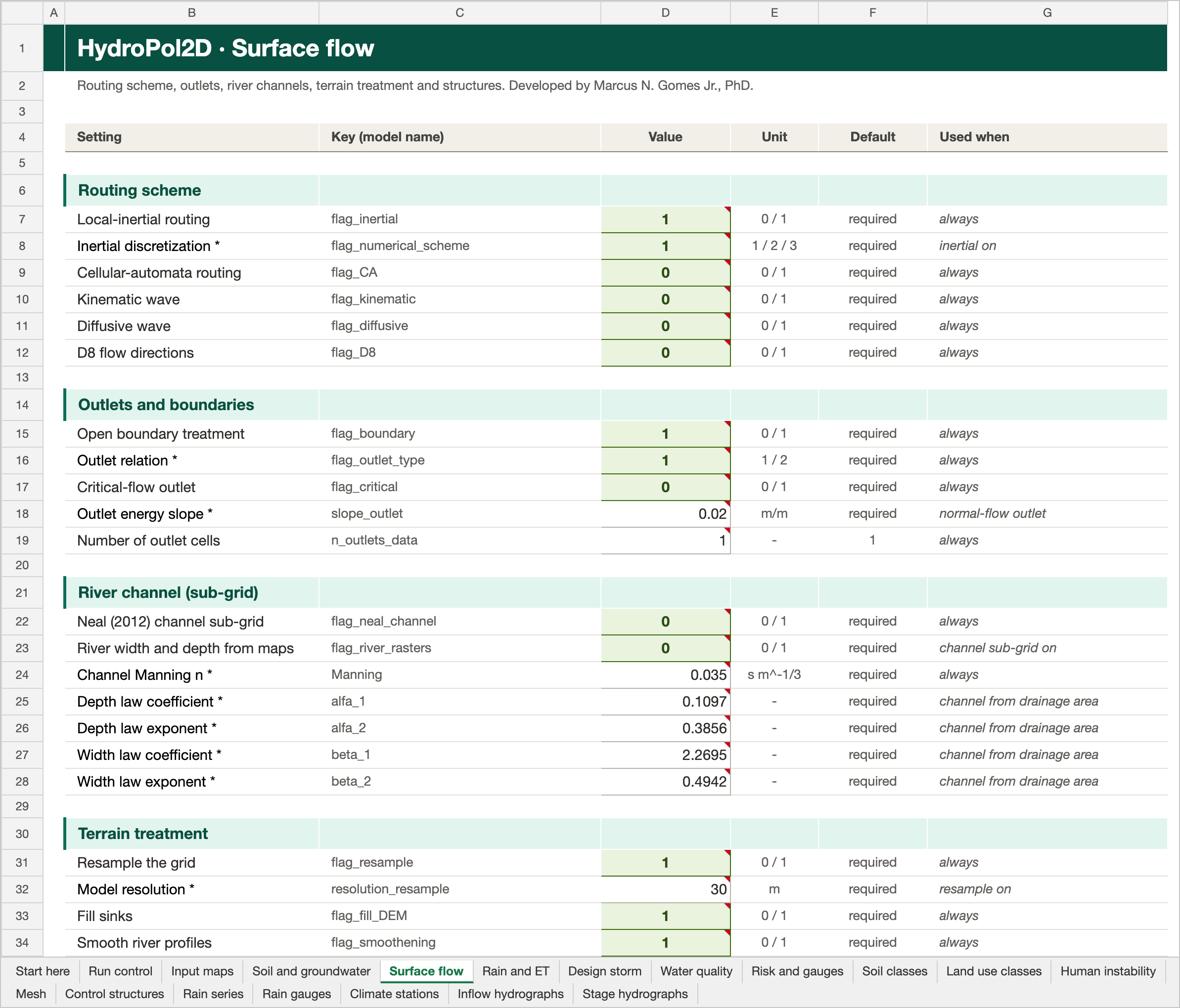
The Surface flow tab of the Stanford example workbook. Click the picture to open it full size.

Routing scheme

Setting	Key	Unit	Default	Used when	Description
Local-inertial routing	flag_inertial	0 / 1	required	always	Selects the local-inertial hydrodynamic solver. It is the required routing solver for the active Neal (2012) channel-subgrid extension.
Inertial discretization	flag_numerical_scheme	1 / 2 / 3	required	inertial on	Chooses the local-inertial discretization: 1 = Bates, 2 = slope-upwind, 3 = slope-centered. The value is used only by routing options that call the inertial scheme.
Cellular-automata routing	flag_CA	0 / 1	required	always	Selects the cellular-automata hydrodynamic routing option. Do not enable it together with local inertial or full momentum routing.
Kinematic wave	flag_kinematic	0 / 1	required	always	Selects the kinematic-wave routing alternative. Do not combine it with local inertial, full momentum, or cellular automata routing.
Diffusive wave	flag_diffusive	0 / 1	required	always	Selects the diffusive-wave routing alternative. Do not combine it with local inertial, full momentum, or cellular automata routing.
D8 flow directions	flag_D8	0 / 1	required	always	Retired: keep at 0. The old raster D8 was incomplete, and 1 stops the run. D8 local-inertial routing is flag_d8_local_inertial, set in the bypass script (see Limitations).

Outlets and boundaries

Setting	Key	Unit	Default	Used when	Description
Open boundary treatment	flag_boundary	0 / 1	required	always	Activates the configured open/perimeter boundary treatment. Define the outlet mask and outlet slope carefully because this setting controls water removal at the domain edge.
Outlet relation	flag_outlet_type	1 / 2	required	always	Chooses the outlet relation: 1 = normal-flow outlet using slope_outlet; 2 = critical-flow outlet. The selected outlet cells determine where this relation is applied.
Critical-flow outlet	flag_critical	0 / 1	required	always	Uses the critical-flow outlet treatment where the selected routing solver supports it. This is distinct from the normal-flow outlet selected with flag_outlet_type.
Outlet energy slope	slope_outlet	m/m	required	normal-flow outlet	slope_outlet is the positive normal-flow energy slope in m/m applied at configured outlet cells. It should represent the downstream channel or terrain gradient beyond the modeled domain.
Number of outlet cells	n_outlets_data	-	1	always	n_outlets_data is the number of domain-edge cells used as outlets (rounded, at least 1). Outlets grow from the lowest perimeter cell unless an outlet-cell CSV is supplied. Default 1.

River channel (sub-grid)

Setting	Key	Unit	Default	Used when	Description
Neal (2012) channel sub-grid	flag_neal_channel	0 / 1	required	always	Activates the Neal (2012) embedded rectangular channel and floodplain extension. It requires flag_inertial = 1, structured raster topology, and valid river-width and river-depth rasters.
River width and depth from maps	flag_river_rasters	0 / 1	required	channel sub-grid on	Uses supplied RiverWidths and RiverDepths rasters to define the channel geometry for the active subgrid model.
Channel Manning n	Manning	s m^-1/3	required	always	Manning is the in-bank channel Manning roughness in s m^-1/3, applied on river cells. Land and overbank cells use the the Land use classes tab roughness.
Depth law coefficient	alfa_1	-	required	channel from drainage area	alfa_1 is the coefficient in the derived channel-depth relation H = alfa_1 A^alfa_2, where A is contributing area in km2. It is used only when channel geometry is derived rather than supplied as rasters.
Depth law exponent	alfa_2	-	required	channel from drainage area	alfa_2 is the exponent in the derived channel-depth relation H = alfa_1 A^alfa_2. Use a value calibrated or justified for the target river network.
Width law coefficient	beta_1	-	required	channel from drainage area	beta_1 is the coefficient in the derived channel-width relation W = beta_1 A^beta_2, where A is contributing area in km2. It is bypassed by supplied river-width rasters.
Width law exponent	beta_2	-	required	channel from drainage area	beta_2 is the exponent in the derived channel-width relation W = beta_1 A^beta_2. It controls how quickly generated channels widen downstream.

Terrain treatment

Setting	Key	Unit	Default	Used when	Description
Resample the grid	flag_resample	0 / 1	required	always	Resamples ancillary rasters to the DEM grid during preprocessing when their grid differs from the DEM.
Model resolution	resolution_resample	m	required	resample on	resolution_resample is the working model-grid resolution in metres when raster resampling is enabled. All model inputs are aligned to this resolution during preprocessing.
Fill sinks	flag_fill_DEM	0 / 1	required	always	Fills terrain depressions before deriving drainage directions and flow accumulation.
Smooth river profiles	flag_smoothening	0 / 1	required	always	Applies constrained stream-profile smoothing during DEM preprocessing. This option requires Optimization Toolbox.
Stream threshold area	min_area	km2	required	smoothing on	min_area is the contributing-area threshold in km2 used to extract the modeled stream network and derive hydraulic geometry from flow accumulation.
Smoothing strength	K_value	0 to 20	required	smoothing on	K_value is the smoothing strength passed to the constrained regularized stream-profile smoother. It is used only when DEM smoothing is enabled; larger values produce stronger profile regularization.
Smoothing regularization	tau	0 to 1	required	smoothing on	tau is the dimensionless regularization setting passed to the constrained regularized stream-profile smoother. It is used only when DEM smoothing is enabled.
Minimum imposed slope	sl	m/m	required	smoothing on	sl is the minimum imposed drainage gradient in m/m used by terrain conditioning when minimum-slope imposition is enabled.
Smooth cells	flag_smooth_cells	0 / 1	required	always	Applies the configured cell-level DEM smoothing treatment during preprocessing.
Trunk streams only	flag_trunk	0 / 1	required	always	Uses the trunk-stream processing option during terrain and drainage-network preparation.
Reduce the DEM	flag_reduce_DEM	0 / 1	required	always	Applies the configured river-channel DEM reduction during preprocessing.
DTM filter	flag_DTM	0 / 1	required	always	Uses the DTM-processing pathway for terrain preparation when that workflow is required by the input data.
DTM filter slope	slope_DTM	%	required	DTM filter on	slope_DTM is the slope threshold in percent used by the DTM filter. It is read only when the DTM filtering option is enabled.

Unstructured mesh

Setting	Key	Unit	Default	Used when	Description
Voronoi mesh	flag_voronoi	0 / 1	0	always	Runs the model on a prepared Voronoi (unstructured) mesh instead of the raster grid. Mesh options are read from the Mesh tab.
Voronoi sub-grid tables	flag_voronoi_subgrid	0 / 1	required	Voronoi on	Enables sub-grid face tables (stage versus flow area, wetted perimeter and conveyance) on the Voronoi mesh. Used only with flag_voronoi = 1; the table path is set in the Mesh tab.

Inflows and structures

Setting	Key	Unit	Default	Used when	Description
Inflow hydrographs	flag_inflow	0 / 1	required	always	Applies one or more prescribed discharge hydrographs at the inlet coordinates defined in the Inflow hydrographs tab.
Stage hydrographs	flag_stage_hydrograph	0 / 1	required	always	Applies a prescribed water-level hydrograph at the configured stage-boundary location(s).
Reservoirs	flag_reservoir	0 / 1	required	always	Enables the reservoir and control-structure module using the configured reservoir inputs.

Paused (keep at 0: setting 1 stops the run)

Setting	Key	Unit	Default	Used when	Description
Lookup-table sub-grid (paused)	flag_structured_lookup_subgrid	0 / 1	0	paused	Enables the structured lookup-table subgrid formulation on the regular raster model. It uses level-dependent cell and face properties and cannot be combined with Neal or Voronoi subgrid.
High-resolution DEM for that sub-grid (paused)	Subgrid_DEM_path	m	empty	paused	Subgrid_DEM_path is an optional high-resolution DEM GeoTIFF in metres for the lookup-table sub-grid. It is read only when the lookup sub-grid is on without overbank mode.

Rain and ET

Where rainfall and evapotranspiration come from, and the lists of map files.

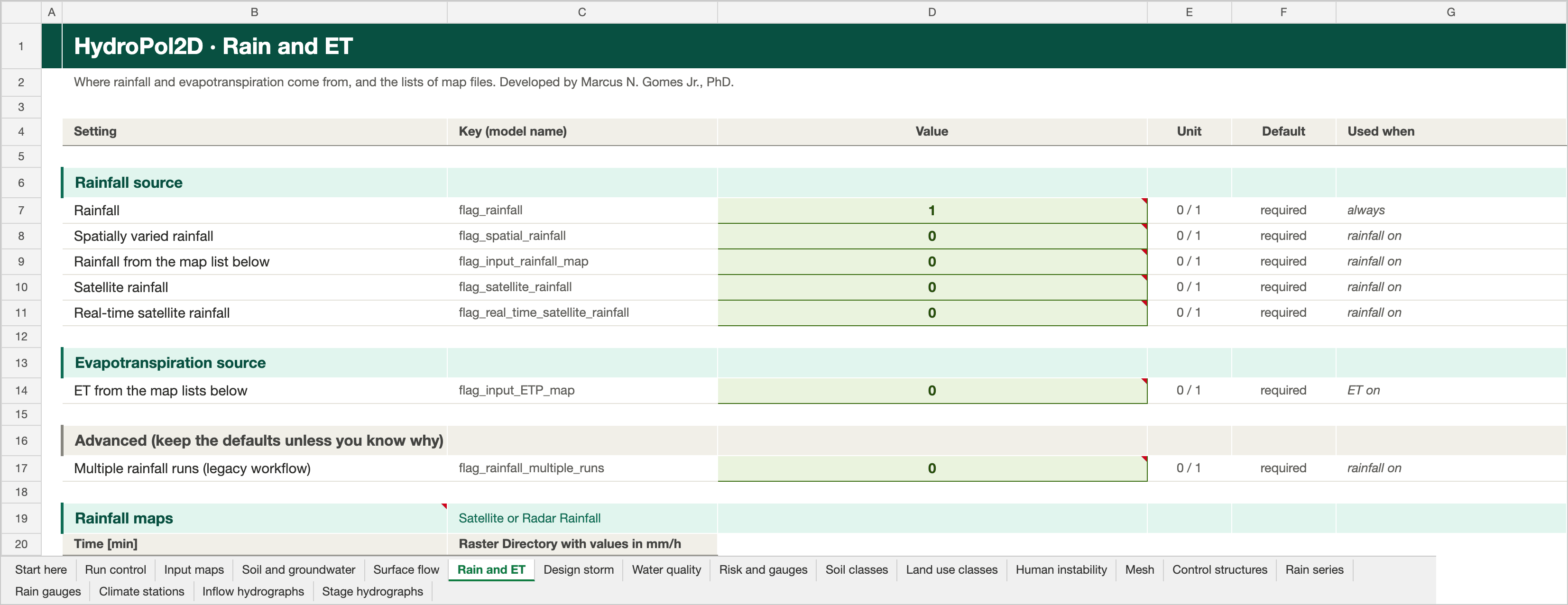
The Rain and ET tab of the Stanford example workbook. Click the picture to open it full size. The picture ends at the column titles of the first map list.

Rainfall source

Setting	Key	Unit	Default	Used when	Description
Rainfall	flag_rainfall	0 / 1	required	always	Enables rainfall forcing. Use this with one selected rainfall source: a lumped time series, gauge interpolation, a scheduled raster sequence, or a satellite product.
Spatially varied rainfall	flag_spatial_rainfall	0 / 1	required	rainfall on	Interpolates rainfall from the configured rainfall gauges to every model cell. Gauge coordinates and a common rainfall time series are required.
Rainfall from the map list below	flag_input_rainfall_map	0 / 1	required	rainfall on	Reads a time-indexed sequence of rainfall rasters from the Rainfall maps list. Do not enable this together with another spatial-rainfall source.
Satellite rainfall	flag_satellite_rainfall	0 / 1	required	rainfall on	Activates the satellite-rainfall forcing workflow. It prepares an hourly spatial-rainfall schedule and enables rainfall automatically.
Real-time satellite rainfall	flag_real_time_satellite_rainfall	0 / 1	required	rainfall on	Activates the real-time satellite rainfall workflow. This experimental option creates a short rolling spatial-rainfall schedule.

Evapotranspiration source

Setting	Key	Unit	Default	Used when	Description
ET from the map lists below	flag_input_ETP_map	0 / 1	required	ET on	Reads paired transpiration and evaporation raster schedules from the Rain and ET tab. Both schedules must have the same time entries.

Advanced (keep the defaults unless you know why)

Setting	Key	Unit	Default	Used when	Description
Multiple rainfall runs (legacy workflow)	flag_rainfall_multiple_runs	0 / 1	required	rainfall on	Activates the legacy multiple-rainfall-run workflow. Leave disabled for one standard rainfall event.

Design storm

Synthetic storms from a local IDF relation i = K RP^a / (b + duration)^c.

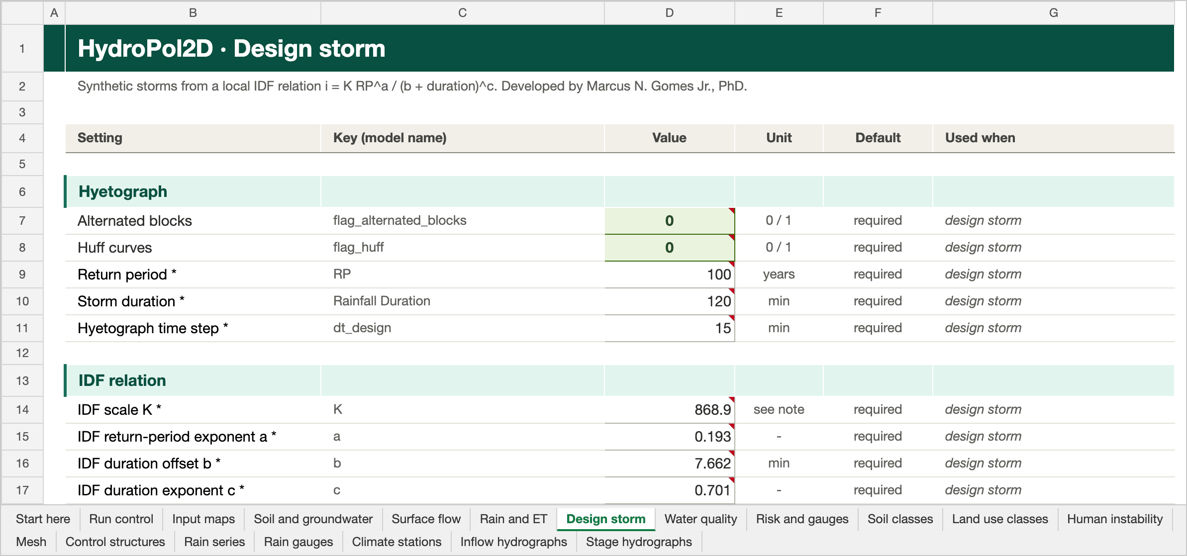
The Design storm tab of the Stanford example workbook. Click the picture to open it full size.

Hyetograph

Setting	Key	Unit	Default	Used when	Description
Alternated blocks	flag_alternated_blocks	0 / 1	required	design storm	Generates the configured alternating-block design storm instead of reading a rainfall time series.
Huff curves	flag_huff	0 / 1	required	design storm	Generates the configured Huff design storm instead of reading a rainfall time series.
Return period	RP	years	required	design storm	RP is the design-storm return period in years. It is used by the selected IDF relation to calculate rainfall intensity.
Storm duration	Rainfall Duration	min	required	design storm	Rainfall Duration is the total design-storm duration in minutes. It sets the length of the generated Alternated Blocks or Huff hyetograph.
Hyetograph time step	dt_design	min	required	design storm	dt_design is the time increment in minutes used to discretize the generated design hyetograph. It should be short enough to resolve the intended rainfall peak.

IDF relation

Setting	Key	Unit	Default	Used when	Description
IDF scale K	K	see note	required	design storm	K is the scale coefficient of the local IDF relation i = K RP^a / (b + duration)^c. Its units must be consistent with intensity in mm/h and duration in minutes.
IDF return-period exponent a	a	-	required	design storm	a is the dimensionless return-period exponent in the local IDF relation. Use coefficients fitted for the study location.
IDF duration offset b	b	min	required	design storm	b is the duration offset in the local IDF relation, expressed in minutes when duration is entered in minutes.
IDF duration exponent c	c	-	required	design storm	c is the dimensionless duration exponent in the local IDF relation. It controls how intensity decays as storm duration increases.

Water quality

Pollutant build-up and wash-off.

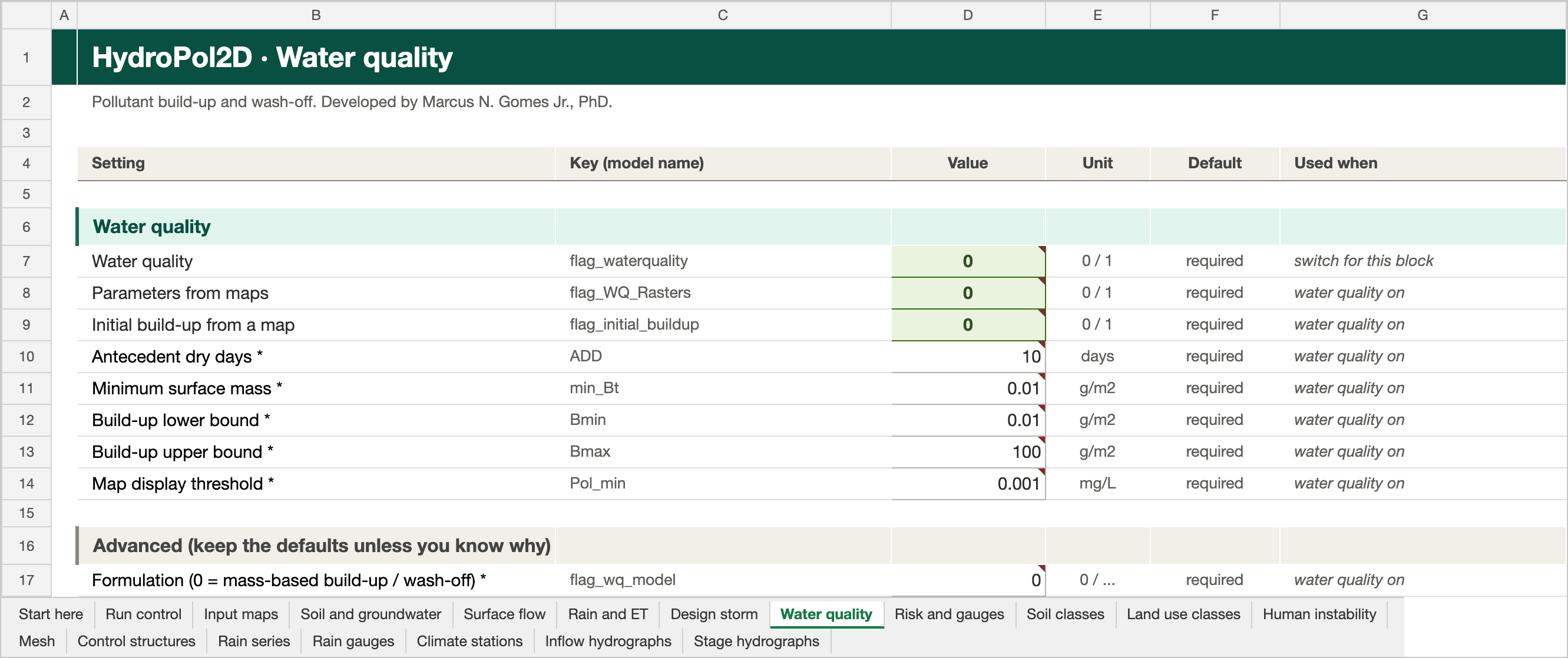
The Water quality tab of the Stanford example workbook. Click the picture to open it full size.

Water quality

Switch: flag_waterquality. The rest of the block greys out while it is 0.

Setting	Key	Unit	Default	Used when	Description
Water quality	flag_waterquality	0 / 1	required	switch for this block	Enables pollutant buildup, washoff, transport, and output calculations.
Parameters from maps	flag_WQ_Rasters	0 / 1	required	water quality on	Uses spatial water-quality coefficient rasters B1, B2, W1, and W2 instead of the land-cover table coefficients.
Initial build-up from a map	flag_initial_buildup	0 / 1	required	water quality on	Initializes water-quality buildup using the configured antecedent dry-period and buildup settings.
Antecedent dry days	ADD	days	required	water quality on	ADD is antecedent dry days. When no initial-buildup raster is used, it enters the exponential buildup initialization B0 = C1 [1 - exp(-C2 ADD)].
Minimum surface mass	min_Bt	g/m2	required	water quality on	min_Bt is the minimum pollutant surface mass density in g/m2 retained by the water-quality washoff calculation. It prevents numerical treatment of negligible pollutant mass.
Build-up lower bound	Bmin	g/m2	required	water quality on	Bmin is the lower pollutant buildup bound in g/m2 used by the selected buildup/washoff formulation. Use a nonnegative value no larger than Bmax.
Build-up upper bound	Bmax	g/m2	required	water quality on	Bmax is the upper pollutant buildup bound in g/m2 used by the selected buildup/washoff formulation. It limits physically stored pollutant mass where that option is active.
Map display threshold	Pol_min	mg/L	required	water quality on	Pol_min is the minimum pollutant concentration in mg/L displayed in water-quality maps. It is a visualization threshold; values below it are hidden in plots but are not removed from the mass balance.

Advanced (keep the defaults unless you know why)

Greyed out while flag_waterquality is 0.

Setting	Key	Unit	Default	Used when	Description
Formulation (0 = mass-based build-up / wash-off)	flag_wq_model	0 / ...	required	water quality on	Selects the water-quality formulation. Value 0 uses the mass-based buildup/washoff mode; use other values only for supported legacy configurations.

Risk and gauges

Human-instability risk and observation points.

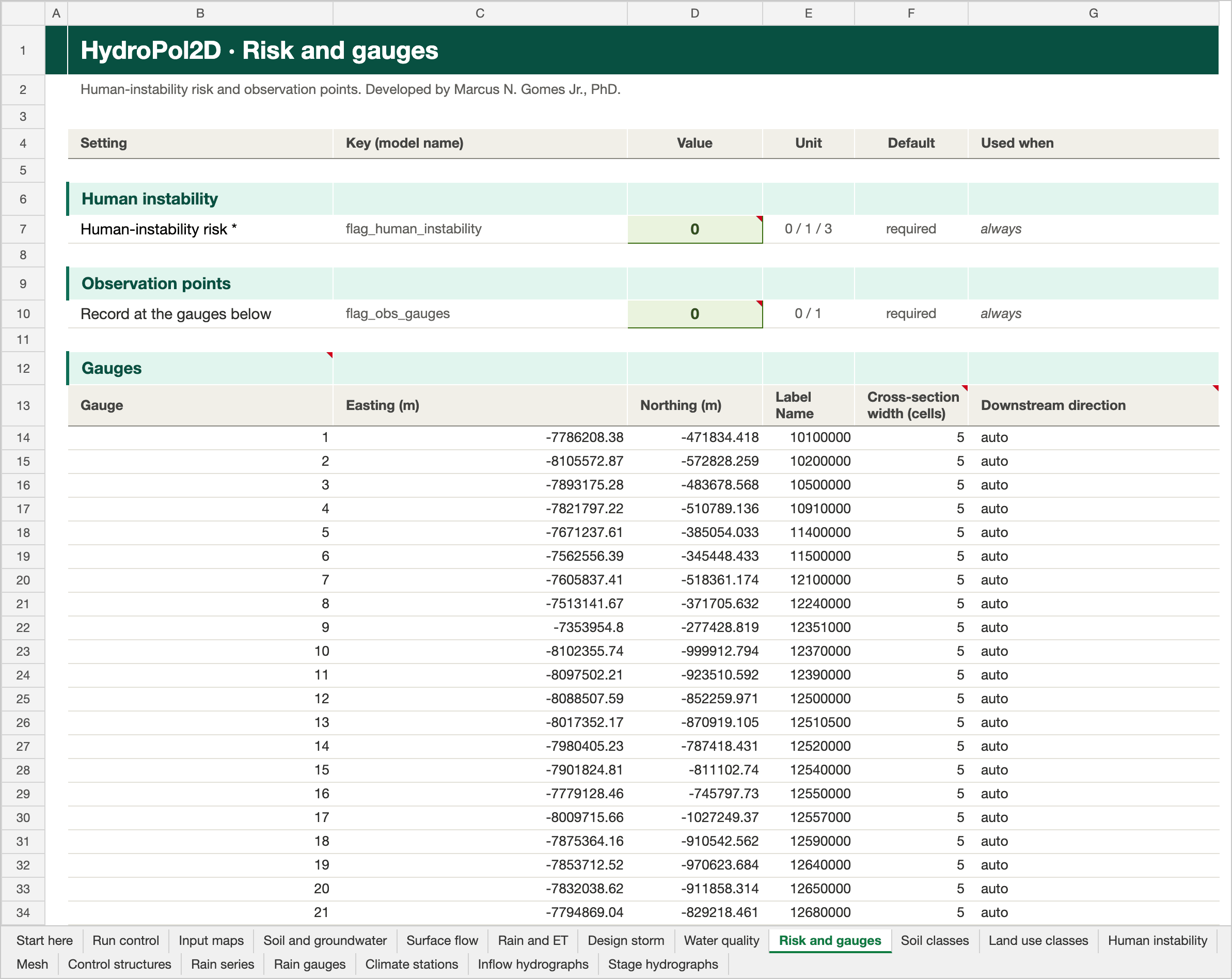
The Risk and gauges tab of the Stanford example workbook. Click the picture to open it full size.

Human instability

Setting	Key	Unit	Default	Used when	Description
Human-instability risk	flag_human_instability	0 / 1 / 3	required	always	Calculates depth-velocity human-instability indicators. Value 0 disables it; value 1 uses the basic classification and value 3 enables the extended classification.

Observation points

Setting	Key	Unit	Default	Used when	Description
Record at the gauges below	flag_obs_gauges	0 / 1	required	always	Exports modeled values at the observation-gauge coordinates listed in the gauge table.

---

Gauge table and discharge cross-sections

With flag_obs_gauges = 1, the model records results at each gauge of the gauge table on the Risk and gauges tab.

Column	Required	Meaning
Gauge	yes	Gauge number
Easting (m), Northing (m)	yes	Gauge position, in the DEM projection
Label Name	yes	Name used in the outputs
Cross-section width (cells)	no	Number of cells in the discharge cross-section. Empty: 5. An even width is raised by 1, so the gauge stays in the middle.
Downstream direction	no	auto (default), or N, S, E, W

The table ends at the first empty row.

What a gauge records. Depth and water level are taken at the gauge cell. Discharge is summed across a cross-section, a line of cells across the flow and centred on the gauge cell:

1. With auto, the downstream direction is downhill along the mean terrain gradient over a width × width window around the gauge. Use N, S, E or W where the terrain is flat. N or S gives an east-west line; E or W gives a north-south line.
2. Cells outside the grid or the domain are dropped from the line.
3. The discharge is the signed sum over the downstream faces of the line, the same rule as the HydroPol2D-Python routing gauges. D8 diagonals that cross the line count.
4. Both face conventions of the routing solvers are handled: one-sided outflows (cellular automata, D8 inertial) and signed face fluxes stored on both faces (D4 inertial, diffusive, kinematic, full momentum). Inertial runs are therefore not double counted.

Outputs.

Output	Content
Gauge hydrograph figures	A dash-dot line with the cross-section discharge
Rating_Curve_Gauges.csv	The column Cross-section Discharge (m3/s)
Gauge_Cross_Sections.csv	The grid row and column of every cell of each cross-section

In bypass mode the two optional columns of the gauge CSV are Cross_section_width_cells and Downstream_direction. The checks are in Validation/Gauges/run_gauge_cross_section_checks.m.

---

Bypass mode and environment variables

• In bypass mode the same keys are fields of InputData_Bypass.flags (switches, layered and Feddes settings) and InputData_Bypass.general (other settings, such as the deep-aquifer starting state).
• Environment variables override the workbook. The Case Builder uses them.

Variable	Overrides
HYDROPOL_INPUT_EXCEL_FILE	The workbook to read
HYDROPOL_SUBSURFACE_SCHEME, HYDROPOL_ENABLE_FEDDES, HYDROPOL_IMPLICIT_WATER_TABLE_FLUX	The layered, Feddes and implicit-flux switches
HYDROPOL_<NAME>	Any numeric layered or Feddes setting, by its key in capitals
HYDROPOL_DEEP_INITIAL_BASEFLOW_MM_DAY, HYDROPOL_DEEP_MEAN_RECHARGE_MM_YEAR, HYDROPOL_DEEP_INITIAL_STATE_PATH	The deep-aquifer starting state
HYDROPOL_SOIL_LATERAL_CONDUCTIVITY_MULTIPLIER, HYDROPOL_REGOLITH_LATERAL_CONDUCTIVITY_MULTIPLIER	The fitted lateral-conductivity multipliers

---

Older layout

Cases made before 2026-10-20 use General_Data.xlsx with its Flags sheet and separate workbooks. They still run unchanged. Each reader takes its tab from the case workbook when the case has one, and the older workbook otherwise.

Case workbook	Older layout
Eight settings tabs	The General_Data sheet: settings in blocks, raster paths in columns T and U
Switches inside their blocks	The Flags sheet: one switch per row, value in column E
Soil classes, Land use classes, Human instability, Mesh, Control structures	SOIL_parameters.xlsx, LULC_parameters.xlsx, human_risk.xlsx, Voronoi_Settings.xlsx, BC_Control_structure.xlsx
Rain series, Rain gauges, Climate stations, Inflow hydrographs, Stage hydrographs	Rainfall_Intensity_Data.xlsx, Rainfall_Spatial_Input.xlsx, ETP_input_data.xlsx, Inflow_Hydrograph.xlsx, Stage_Hydrograph.xlsx

To convert an older case, run the workbook builder from tools/workbook_builder in the MATLAB repository:

python build_input_workbook.py input_catalog.yaml General_Data.xlsx HydroPol2D_Inputs.xlsx

It carries every value, map path, map list and gauge over, and copies the class tables and series from the workbooks next to the source. A series that the case's switches do not read is kept as an empty template with its headers. The V-tilted case gives identical results from either layout (Validation/Workbook/run_single_workbook_checks.m).

The older workbooks no longer need the retired switches flag_data_source, flag_dam_break and flag_river_heigth_compensation (all default 0). flag_subgrid and flag_overbanks are derived from the channel switches, and time_save_ETP is optional.