Groundwater Model

1. Overview

The groundwater component of HydroPol2D represents the coupled dynamics of:

• vadose-zone storage,
• recharge from infiltration,
• lateral saturated groundwater flow,
• groundwater exfiltration to the surface,
• and groundwater interaction with river cells.

The current implementation combines three complementary components:

1. a layered vadose/recharge module, which moves water through near-surface, root-zone, and transmission-zone storage using a reduced Richards-consistent Darcy closure based on the van Genuchten–Mualem constitutive relations,

2. a capillary-rise exchange module, which can move water upward from shallow groundwater into available vadose storage, and

3. a two-dimensional Boussinesq groundwater flow solver, which routes saturated flow laterally across the domain and returns exfiltration to the land surface when the groundwater table rises above the local surface elevation.

This structure allows HydroPol2D to represent dynamic coupling between:

• surface water,
• vadose storage,
• groundwater recharge,
• saturated groundwater flow,
• and saturation-excess return flow.

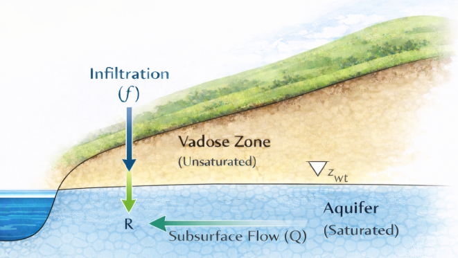
Figure 1. Conceptual representation of the aquifer component in HydroPol2D.

---

2. General Conceptual Structure

The groundwater model is coupled with two clocks. Vadose-zone exchange is evaluated every surface-water time step because infiltration and evapotranspiration need fast soil-moisture feedback. Saturated groundwater heads are updated less frequently, usually on a daily target time step unless stability or head-change limits require a shorter update.

The logic is:

1. compute the water table position from the current groundwater head,
2. determine the maximum unsaturated storage permitted by the current water table depth,
3. compute drainage/recharge from vadose layers to groundwater during the current surface step,
4. compute capillary rise from groundwater to the vadose layers when enabled,
5. accumulate the net exchange volume in the groundwater scheduler,
6. update saturated groundwater heads when the scheduler is due,
7. solve lateral groundwater flow using a 2D Boussinesq equation when baseflow is active,
8. compute groundwater exfiltration to the surface,
9. correct vadose storage if the rising water table reduces the available unsaturated storage,
10. update surface water depth accordingly.

The principal variables are:

• $h$ = groundwater hydraulic head $[\mathrm{L}]$
• $z_0$ = aquifer base elevation or bedrock elevation $[\mathrm{L}]$
• $H = h - z_0$ = saturated thickness $[\mathrm{L}]$
• $R$ = recharge rate to groundwater $[\mathrm{L}\,\mathrm{T}^{-1}]$
• $q_{\mathrm{exf}}$ = exfiltration flux from groundwater to the surface $[\mathrm{L}\,\mathrm{T}^{-1}]$
• $S_y$ = specific yield $[-]$
• $K$ = saturated hydraulic conductivity $[\mathrm{L}\,\mathrm{T}^{-1}]$

2.1 Asynchronous scheduler

The asynchronous scheduler is active by default when groundwater modeling is enabled. The principal controls are:

Control	Default	Meaning
flag_groundwater_async	1	Uses slower saturated-groundwater updates instead of updating heads every surface step.
groundwater_target_dt_min	1440	Target groundwater update interval, in minutes.
groundwater_min_dt_min	1	Minimum groundwater update interval, in minutes.
groundwater_max_head_change_m	0.25	Forces an update when accumulated exchange would change head by this amount.
groundwater_courant	0.25	Stability factor for the Boussinesq groundwater timestep estimate.
flag_capillary_rise	1	Enables simple layered capillary rise when layered soil storage is present.

Pending recharge, capillary rise, and net exchange are stored as scheduler state variables. When a groundwater update runs, the accumulated net exchange depth is divided by the elapsed groundwater interval to form the recharge term passed to the saturated solver.

---

3. Water Table Position and Unsaturated-Zone Capacity

HydroPol2D determines the position of the water table relative to the land surface using the current groundwater head.

Let:

• $z_{\mathrm{surf}}$ = land-surface elevation $[\mathrm{L}]$
• $D_{\mathrm{soil}}$ = soil depth $[\mathrm{L}]$
• $h$ = groundwater hydraulic head $[\mathrm{L}]$

The saturated thickness above the bedrock is computed as

$$z_{\mathrm{gw}} = h - \left(z_{\mathrm{surf}} - D_{\mathrm{soil}}\right)$$

The depth from the land surface to the water table is then

$$z_{\mathrm{wt}} = D_{\mathrm{soil}} - z_{\mathrm{gw}}$$

with the constraint

$$z_{\mathrm{wt}} \ge 0$$

where:

• $z_{\mathrm{gw}}$ = saturated thickness measured upward from the aquifer base $[\mathrm{L}]$
• $z_{\mathrm{wt}}$ = depth to water table below the ground surface $[\mathrm{L}]$

This variable is central to the coupling between vadose storage and groundwater.

3.1 Maximum unsaturated storage

The maximum water that can be stored in the unsaturated zone is defined using the current active storage above residual water content convention:

$$S_{\mathrm{UZ,max}} = z_{\mathrm{wt}} \left( \theta_{\mathrm{sat}} - \theta_r \right)$$

where:

• $S_{\mathrm{UZ,max}}$ = maximum unsaturated storage $[\mathrm{L}]$
• $\theta_{\mathrm{sat}}$ = saturated volumetric water content $[-]$
• $\theta_r$ = residual volumetric water content $[-]$

Thus, as the water table rises, the vadose zone shrinks and the storage capacity available for infiltration decreases. When layered soil storage is active, the code evaluates this limit through the explicit capacities of the near-surface, root-zone, and transmission-zone stores after truncation by the current water-table position.

---

4. Default Layered Vadose-to-Groundwater Exchange

Recharge is computed from the current vadose storage after the infiltration module has already moved water from the surface into the soil. This avoids double-counting infiltration. The current default pathway is layered:

• near-surface storage,
• root-zone storage,
• transmission-zone storage,
• groundwater recharge.

4.1 Surface-step coupling

Vadose exchange is evaluated every surface-water step because infiltration and evapotranspiration need immediate soil-moisture feedback. In the current implementation, infiltration is first accepted by the infiltration module, stored in the vadose layers, and only then allowed to drain downward toward groundwater.

4.2 Layerwise constitutive state

For a generic vadose layer $\ell$ with active storage $S_{\ell}$ and thickness $z_{\ell}$, HydroPol2D evaluates

$$\theta_{\ell} = \theta_{\mathrm{r},\ell} + \frac{S_{\ell}}{z_{\ell}}$$ $$S_{e,\ell} = \frac{ \theta_{\ell} - \theta_{\mathrm{r},\ell} }{ \theta_{\mathrm{sat},\ell} - \theta_{\mathrm{r},\ell} }$$ $$K_{\ell} = K_{\mathrm{sat},\ell} S_{e,\ell}^{\ell_v} \left[ 1 - \left(1 - S_{e,\ell}^{1/m_{\ell}}\right)^{m_{\ell}} \right]^2$$

with

$$m_{\ell} = 1 - \frac{1}{n_{\ell}}$$

where:

• $\theta_{\ell}$ = layer water content $[-]$
• $S_{e,\ell}$ = layer effective saturation $[-]$
• $K_{\ell}$ = layer unsaturated conductivity $[\mathrm{L}\,\mathrm{T}^{-1}]$
• $\ell_v$ = Mualem pore-connectivity parameter $[-]$

This is the same van Genuchten-Mualem constitutive family used by the infiltration module.

4.3 Downward drainage cascade

The layered recharge pathway is computed as a downward cascade:

1. near-surface drainage goes to the root zone when root storage exists,
2. root-zone drainage goes to the transmission zone when transmission storage exists,
3. transmission-zone drainage becomes groundwater recharge.

Conceptually, the drainage depth from a layer over a time step can be summarized as

$$\Delta D_{\ell} \approx K_{\ell}\,\Delta t$$

subject to:

• water available in the donor layer,
• remaining capacity in the receiving layer,
• and the current layer thickness and soil parameters.

The net downward recharge reaching groundwater is then

$$R_{\mathrm{down}} = \frac{\Delta S_{\rightarrow \mathrm{gw}}}{\Delta t}$$

where $\Delta S_{\rightarrow \mathrm{gw}}$ is the total transmission of water into groundwater during the current surface step. Direct drainage from the near-surface or root zone to groundwater occurs only when the lower vadose layers are absent.

4.4 Legacy fallback formulation

HydroPol2D still contains the older representative-bucket recharge closure for cases where the explicit layered storage data are unavailable. In that fallback mode, a single vadose storage state is converted to a representative water content and drained with a Darcy-like closure. That formulation should be treated as legacy/fallback, not the primary theory path for the current model.

---

5. Optional Capillary Rise

When flag_capillary_rise = 1, HydroPol2D allows shallow groundwater to move upward into available vadose storage. The current implementation is a simple layered capillary-rise rule, not a full Richards-equation solution.

The upward exchange increases with:

• shallower water-table depth,
• larger storage deficit in the receiving layer,
• and larger saturated conductivity in that layer.

Conceptually, the upward capillary transfer into layer $\ell$ is limited by

$$C_{\ell} \le \min\!\left( S_{\ell,\mathrm{def}},\, K_{\mathrm{sat},\ell} f_{\mathrm{prox}}(z_{\mathrm{wt}}) f_{\mathrm{dry}}(S_{\ell}) \right)$$

where:

• $S_{\ell,\mathrm{def}}$ is the remaining layer storage deficit
• $f_{\mathrm{prox}}$ is a monotonic water-table proximity factor
• $f_{\mathrm{dry}}$ is a monotonic dryness factor

In the current code, capillary rise is evaluated first into the transmission zone, then the root zone, and only into the near-surface layer when no lower vadose storage exists.

The net vadose-groundwater exchange accumulated by the scheduler is therefore

$$R_{\mathrm{net}} = R_{\mathrm{down}} - C_{\mathrm{up}}$$

where $C_{\mathrm{up}}$ is the total upward capillary-rise flux.

---

6. Two-Dimensional Boussinesq Groundwater Flow Model

Once recharge has been computed, HydroPol2D routes groundwater laterally using the function Boussinesq_2D_explicit.

This solver represents the saturated groundwater system through a depth-integrated unconfined flow approximation.

6.1 Governing equation

The groundwater routing follows the 2D Boussinesq equation in conservative form:

$$S_y \frac{\partial h}{\partial t} = - \nabla \cdot \mathbf{F} + R$$

where:

• $S_y$ = specific yield $[-]$
• $h$ = groundwater hydraulic head $[\mathrm{L}]$
• $\mathbf{F}$ = groundwater flux vector $[\mathrm{L}^2\,\mathrm{T}^{-1}]$
• $R$ = recharge rate $[\mathrm{L}\,\mathrm{T}^{-1}]$

HydroPol2D evaluates this equation numerically by computing fluxes at cell interfaces and then updating the groundwater head explicitly.

6.2 Saturated thickness

The active saturated thickness is defined as

$$H = \max(h - z_0, 0)$$

where:

• $H$ = saturated thickness $[\mathrm{L}]$
• $z_0$ = aquifer base elevation or bedrock elevation $[\mathrm{L}]$

This enforces the physical condition that no saturated storage exists below the aquifer base.

6.3 Interface fluxes

HydroPol2D computes groundwater fluxes at cell interfaces using Darcy’s law with saturated thickness weighting.

For the $x$ direction:

$$F_x = -K_x H_x \frac{\partial h}{\partial x}$$

and for the $y$ direction:

$$F_y = -K_y H_y \frac{\partial h}{\partial y}$$

where:

• $F_x, F_y$ = fluxes per unit width $[\mathrm{L}^2\,\mathrm{T}^{-1}]$
• $K_x, K_y$ = hydraulic conductivity at cell interfaces $[\mathrm{L}\,\mathrm{T}^{-1}]$
• $H_x, H_y$ = interface saturated thicknesses $[\mathrm{L}]$

In the implementation, the interface hydraulic conductivity is taken as the arithmetic average of the conductivities in adjacent cells:

$$K_x = \frac{K_i + K_{i+1}}{2} \qquad K_y = \frac{K_j + K_{j+1}}{2}$$

and the interface saturated thickness is likewise averaged:

$$H_x = \frac{H_i + H_{i+1}}{2} \qquad H_y = \frac{H_j + H_{j+1}}{2}$$

6.4 Conservative flux limiting

To avoid numerical instability and nonphysical depletion of groundwater storage, HydroPol2D applies a flux limiter so that no cell can lose more water than it contains during a substep.

For example, in the $x$ direction, the maximum allowed flux is

$$F_{x,\max} = \frac{S_y H_{\mathrm{donor}}}{\Delta t}$$

and the final interface flux is limited as

$$F_x \leftarrow \operatorname{sign}(F_x)\, \min\left(|F_x|,\,F_{x,\max}\right)$$

A similar expression is used in the $y$ direction.

This is an important feature of the HydroPol2D groundwater solver because it guarantees local mass admissibility during explicit integration.

6.5 Divergence of groundwater fluxes

The divergence of the flux field is then computed from the interface fluxes as

$$\nabla \cdot \mathbf{F} = \frac{\partial F_x}{\partial x} + \frac{\partial F_y}{\partial y}$$

using conservative finite differences on the raster grid.

6.6 Explicit predictor–corrector update

The Boussinesq solver uses an explicit predictor–corrector strategy.

Predictor step

A first estimate of head is computed using the current fluxes:

$$h^{\ast} = h^t + \frac{\Delta t}{S_y}\left(-\nabla \cdot \mathbf{F}^t\right)$$

Corrector step

Fluxes are recomputed from the predictor state, averaged, and used in the final update:

$$h^{t+\Delta t} = h^t + \frac{\Delta t}{S_y} \left( -\nabla \cdot \mathbf{F}^{\mathrm{avg}} + R \right)$$

where:

• $h^{\ast}$ = predictor hydraulic head $[\mathrm{L}]$
• $h^{t+\Delta t}$ = final hydraulic head after the time step $[\mathrm{L}]$
• $\mathbf{F}^{\mathrm{avg}}$ = average of predictor and corrector interface fluxes

This predictor–corrector procedure improves stability and reduces numerical diffusion relative to a simple explicit Euler update.

---

7. Groundwater Update Timing and Adaptive Time Stepping

HydroPol2D uses a two-level groundwater time-step logic.

7.1 Outer asynchronous scheduler

Vadose exchange is accumulated every surface-water step, but saturated groundwater heads are updated only when the groundwater scheduler is due. The groundwater update interval is the minimum of:

• the user target interval,
• the explicit groundwater stability cap,
• the interval implied by the maximum allowed accumulated head change,
• and the final partial interval at the end of the run.

If flag_groundwater_async = 0, the saturated groundwater update is forced every surface step.

7.2 Explicit groundwater stability cap

The outer scheduler cap is based on an explicit diffusivity estimate for the unconfined Boussinesq equation:

$$D = \frac{K H}{S_y}$$ $$\Delta t_{\mathrm{gw,stable}} = \frac{ C_{\mathrm{gw}} \, L_{\mathrm{grid}}^2 }{ 4 D_{\max} }$$

where:

• $D$ = groundwater diffusivity $[\mathrm{L}^2\,\mathrm{T}^{-1}]$
• $C_{\mathrm{gw}}$ = groundwater Courant/safety factor $[-]$
• $L_{\mathrm{grid}} = \min(\Delta x,\Delta y)$
• $D_{\max}$ = maximum domain diffusivity over the active groundwater cells

This is the cap used by the current estimate_groundwater_stable_timestep logic.

7.3 Inner Boussinesq substepping

When a groundwater update is triggered, the scheduler converts the accumulated net exchange depth into an average recharge rate over the elapsed groundwater interval and passes it to the saturated solver. The Boussinesq solver then advances over that interval using internal predictor-corrector substeps.

Those internal substeps are additionally limited by a velocity-based condition of the form

$$\Delta t_{\mathrm{inner}} \le \min\!\left( \frac{C_v \Delta x}{|u_x|},\, \frac{C_v \Delta y}{|u_y|} \right)$$

where:

• $u_x, u_y$ are Darcy groundwater velocities
• $C_v$ is the internal velocity-based safety factor

The result is a two-level strategy:

1. an outer scheduler cap based on explicit groundwater stability and allowed head change,
2. an inner predictor-corrector substepping loop inside the Boussinesq solver.

---

8. Boundary Conditions

The groundwater solver supports:

• Dirichlet boundary conditions,
• no-flow boundary conditions,
• domain masking.

8.1 Dirichlet boundaries

If a Dirichlet mask is provided, the head is prescribed directly:

$$h = h_{\mathrm{D}}$$

on the selected boundary cells, where:

• $h_{\mathrm{D}}$ = prescribed boundary head $[\mathrm{L}]$

8.2 No-flow boundaries

No-flow boundaries are enforced by zero-gradient conditions at the domain perimeter. In practice, HydroPol2D copies the head from the nearest valid interior neighbor to the perimeter cell, thereby enforcing a discrete Neumann condition.

8.3 Catchment mask

All groundwater calculations are restricted to the valid computational domain. Cells outside the catchment mask are set to NaN.

---

9. Groundwater Exfiltration to the Surface

After updating the groundwater head, HydroPol2D computes exfiltration where the groundwater table rises above the effective land surface.

The surface elevation used for exfiltration is

$$h_{\mathrm{surf}} = z_0 + D_{\mathrm{soil}}$$

where:

• $h_{\mathrm{surf}}$ = effective land-surface elevation for groundwater emergence $[\mathrm{L}]$

Exfiltration is then computed as

$$q_{\mathrm{exf}} = \max\left(0,\,h - h_{\mathrm{surf}}\right) \frac{S_y}{\Delta t}$$

where:

• $q_{\mathrm{exf}}$ = exfiltration flux $[\mathrm{L}\,\mathrm{T}^{-1}]$

This expression means that if groundwater head exceeds the land surface, the excess saturated storage is expelled upward and transferred to the surface water system.

The groundwater head is then clipped so that

$$h \le h_{\mathrm{surf}}$$

which prevents groundwater from remaining above the land surface after exfiltration has been accounted for.

---

10. River–Aquifer Exchange

The current solver interface includes:

• a river mask,
• a river conductance term,
• river stage,
• river bed elevation,

which are designed to support river–aquifer exchange. In the current implementation, the placeholder variable

$$q_{\mathrm{river}}$$

is initialized and carried through the coupling interface as the river-exchange term. This means that the interface is present, but river-aquifer exchange should currently be described as a placeholder/structural hook, not a mature standalone theory claim on the same footing as recharge, lateral groundwater flow, capillary rise, or exfiltration.

---

11. Saturation-Excess Correction After Water Table Rise

After the Boussinesq update, HydroPol2D recomputes the water-table depth and therefore the new maximum unsaturated storage:

$$S_{\mathrm{UZ,max}}^{\,\mathrm{new}} = z_{\mathrm{wt}}^{\,\mathrm{new}} \left( \theta_{\mathrm{sat}} - \theta_r \right)$$

If the updated vadose storage exceeds this new capacity, the excess is returned to the surface as saturation-excess water:

$$S_{\mathrm{excess}} = \max\left( S - S_{\mathrm{UZ,max}}^{\,\mathrm{new}}, 0 \right)$$

The correction is then:

$$S \leftarrow S - S_{\mathrm{excess}}$$

and surface water depth is increased by

$$h_{\mathrm{surf}}^{\,\mathrm{new}} = h_{\mathrm{surf}}^{\,\mathrm{old}} + S_{\mathrm{excess}}$$

In the layered default implementation, the same correction is applied after recomputing the admissible summed vadose-layer capacity. This is a very important part of HydroPol2D because it guarantees mass consistency between the vadose and saturated zones when the water table rises during a time step.

---

12. Coupling Back to Surface Water

The groundwater model feeds back to the surface water system in two ways:

1. exfiltration, through $q_{\mathrm{exf}}$,
2. saturation excess, through $S_{\mathrm{excess}}$.

The surface water depth is updated as

$$d_t = d_t + \Delta t\,q_{\mathrm{exf}}$$

with the appropriate unit conversion in the code from $\mathrm{m}$ to $\mathrm{mm}$.

This means that HydroPol2D allows groundwater to actively influence flood generation and near-surface wetness, rather than treating it as a disconnected lower boundary process.

---

13. Mass Balance

The groundwater solver performs an explicit mass-balance check during each update.

The recharge input volume is

$$V_{\mathrm{recharge}} = \sum R\,\Delta t\,A_{\mathrm{cell}}$$

The exfiltration loss volume is

$$V_{\mathrm{exf}} = \sum q_{\mathrm{exf}}\,\Delta t\,A_{\mathrm{cell}}$$

The groundwater storage change is

$$\Delta V_{\mathrm{storage}} = \sum S_y\,\max(h^{t+\Delta t}-z_0,0)\,A_{\mathrm{cell}} - \sum S_y\,\max(h^t-z_0,0)\,A_{\mathrm{cell}}$$

The mass-balance residual is then

$$\varepsilon_{\mathrm{gw}} = V_{\mathrm{recharge}} - V_{\mathrm{exf}} - \Delta V_{\mathrm{storage}}$$

where:

• $\varepsilon_{\mathrm{gw}}$ = groundwater mass-balance error $[\mathrm{L}^3]$

This quantity is stored as a groundwater diagnostic error in HydroPol2D.

When asynchronous groundwater is active, pending accumulated recharge and capillary exchange are not treated as model loss. They are stored as groundwater exchange-in-transit until the next saturated update consumes the scheduler volume. This distinction is important for interpreting whole-model water-balance diagnostics.

---

14. Summary

The HydroPol2D groundwater model combines:

• a layered vadose-zone recharge module based on a Darcy–van Genuchten–Mualem closure,
• simple capillary rise from shallow groundwater into available vadose storage,
• an asynchronous groundwater scheduler for slower saturated-head updates,
• a 2D Boussinesq groundwater flow model for lateral saturated flow,
• adaptive explicit time stepping,
• surface exfiltration when groundwater rises above the ground surface,
• and a saturation-excess correction that preserves mass when the water table reduces vadose storage capacity.

This structure allows HydroPol2D to represent a dynamically coupled subsurface system in which:

• infiltration does not simply disappear into a static bucket,
• recharge affects groundwater head,
• groundwater flow redistributes water laterally,
• and groundwater can return to the land surface and influence overland flow generation.

The result is a groundwater model that is physically interpretable, mass conservative, and fully integrated with the hydrologic and hydrodynamic architecture of HydroPol2D.