Calibrate
Calibrate fits model parameters to observed discharge, water depths, water levels and groundwater depths with a genetic algorithm or SCE-UA (shuffled complex evolution). It is the fourth workspace on the rail (Cmd+4 on a Mac, Ctrl+4 on Windows). The method, the scores and the settings are explained in Calibration Against Observations.
The page has six sections, in the order they are used.
1. Observed data
Choose a table and paste rows from Excel or a text file (Paste rows), or type them.
| Column | Content |
|---|---|
| Gauge | The series name; rows with the same name form one series |
| Easting, Northing | Optional coordinates, in the model's coordinate system |
| Time | Minutes from the start of the run |
| Value | The observed value, in the units of the table |
| Observation uncertainty | Optional: the measurement error of the value, as one standard deviation in the same units |
There are tables for discharge, water depth, water level, groundwater depth and surface soil moisture. Soil moisture cannot be calibrated yet. How to fill this table lists the columns of the selected table. The rows go into the model as they are pasted; Save writes them to the model file.
2. Observations to match
Each row is one observed series. Tick Use for the series to match.
- Compare with: a routing gauge, an observation point, the model outlet (discharge only) or the cell at the series' coordinates. Gauges and observation points are drawn on Setup > Study area.
- Score: KGE, NSE, NSE of log values, RMSE / standard deviation, peak, volume and timing (discharge), or error / uncertainty (series with uncertainty).
- Weight: Auto gives each kind of observation an equal share. A number sets the weight of the series.
- Changes only: scores the ups and downs, not a constant offset; for wells with an uncertain datum.
- Use uncertainty: weights each value by one over its uncertainty squared, so uncertain values count less. It is on by default when the series has uncertainties.
Ignore observations before sets a warm-up period that is simulated but not scored.
3. Parameters to calibrate
Every parameter this model can calibrate is listed, grouped by process. Tick Free for each parameter the search may change; the others keep the model's values.
- Multipliers (model value ×1) scale the value, the class tables and the raster together, so the map keeps its pattern. Start with a few of them.
- Lower and Upper set the search range and can be edited.
- Group and Show free only shorten the list; the count shows how many are free.
- A note appears when there are many free parameters for the kinds of observation matched.
4. Search settings
Search
- Method: Genetic algorithm (the default) or SCE-UA. SCE-UA suits cheap runs and budgets of thousands of runs. With a few hundred runs of an expensive model the genetic algorithm got further (see Section 6.1 of the method page).
- For SCE-UA: complexes (Auto is the number of free parameters, at least 2), points per complex, simplex size and evolution steps per shuffle (Auto uses the recommended values), maximum runs, and the stop rules on improvement and on convergence.
- For the genetic algorithm: population size (Auto is 10 per free parameter), generations, elite share, tournament size, crossover and mutation probabilities, mutation size and early stop.
- For both: starting population, time limit and random seed.
The line under the settings gives the largest number of model runs and, after a first calibration, an estimate of the time.
Computer
- Runs: Auto (measures one run's memory first), One at a time (each run uses the whole computer) or Several at a time.
- Runs at a time and Threads per run, for Several at a time.
- Use at most: the share of the free memory several runs may take.
- Device: the CPU, or a GPU where the computer has one, with the GPU memory per run.
- Results folder: a new folder next to the model file by default.
- Resume the stopped calibration in this folder continues a calibration that was cancelled or interrupted.
5. Run
Start calibration checks the choices and starts the search in the background; Studio stays usable. The progress bar and the line under it show the generation (GA) or shuffle (SCE-UA), the run and the best score so far, and the log lists every run.
Cancel stops the runs in progress at their next model step. Finished runs are saved, so a resumed calibration does not repeat them.
6. Results
- Summary: the best score (0 is a perfect fit), why the search stopped, the runs and the time taken.
- Best values: each free parameter, its model value, its best value, the range over the best 10 % of the candidates, and whether the data pin it down.
- Fit per series: the error of the current model and of the best run, with the KGE or NSE of the best run.
- Show: all series as small panels, the score per series, the search history, or one series. Each panel shows the observations (with their uncertainty), the current model and the best run.
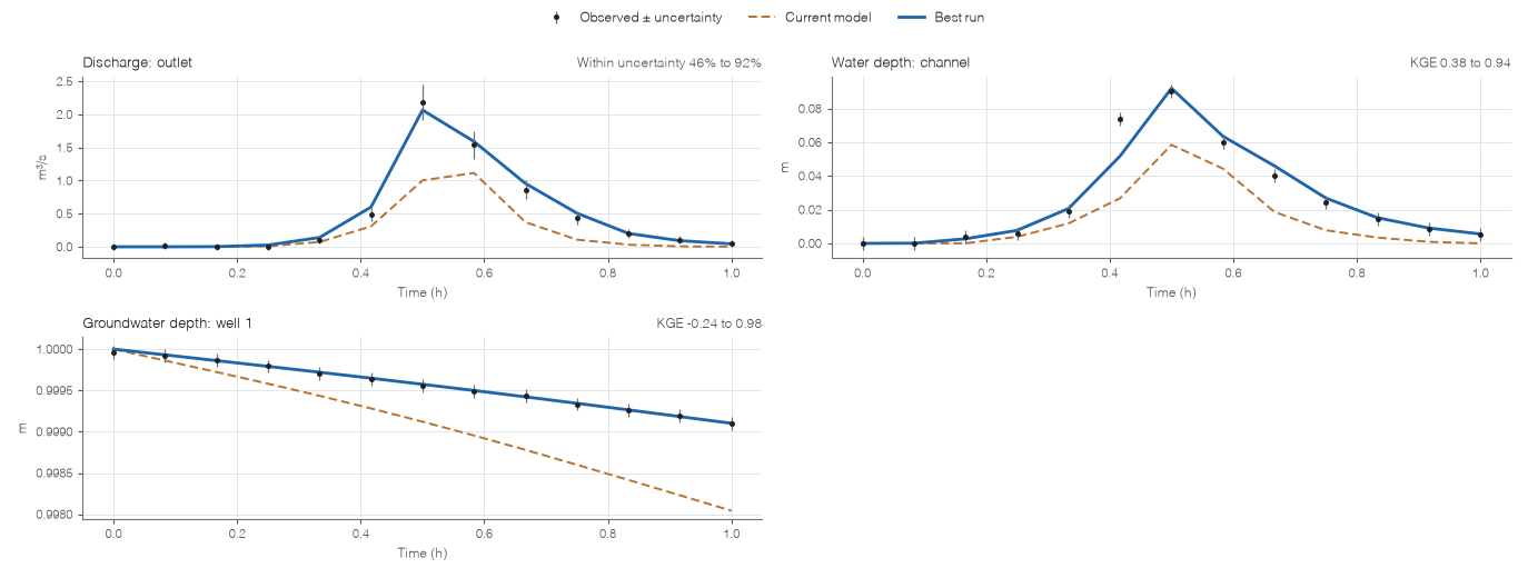
Results of a short calibration: observations with their uncertainty, the current model (dashed) and the best run.
Apply to model writes the best values into the open model; Save keeps them. A multiplier on a raster input writes the scaled raster to the results folder and points the model at it, without changing the original. Undo apply gives the model back as it was, while it has not been edited since. Show results folder opens the folder with the tables and figures of the calibration.