Optional Forcing

HydroPol2D supports several kinds of meteorological and hydrological forcing beyond a single rainfall series. In the MATLAB case workbook HydroPol2D_Inputs.xlsx, the switches sit on the Rain and ET, Design storm, Soil and groundwater and Surface flow tabs, the time series on five series tabs, and the lists of map files on the Rain and ET tab.

---

Where Each Forcing Is Set

Forcing	Switch (tab)	Data
Uniform rainfall series	flag_rainfall (Rain and ET), with no other rainfall source	Rain series tab
Rain gauges, interpolated	flag_spatial_rainfall (Rain and ET)	Rain gauges tab
Rainfall maps	flag_input_rainfall_map (Rain and ET)	Rainfall maps list (Rain and ET tab)
Satellite rainfall	flag_satellite_rainfall, flag_real_time_satellite_rainfall (Rain and ET)	Prepared by the satellite workflow
Design storm	flag_alternated_blocks or flag_huff (Design storm)	Hyetograph and IDF settings on the same tab
Penman–Monteith evapotranspiration	flag_ETP (Soil and groundwater), with no ET maps	Climate stations tab
Evaporation and transpiration maps	flag_input_ETP_map (Rain and ET)	Transpiration maps and Evaporation maps lists (Rain and ET tab)
Inflow hydrographs	flag_inflow (Surface flow)	Inflow hydrographs tab
Stage hydrographs	flag_stage_hydrograph (Surface flow)	Stage hydrographs tab

Use one rainfall source at a time. A series that the case's switches do not read can stay as an empty template with its headers. Every switch and setting is listed on Case Workbook Settings.

---

Rainfall

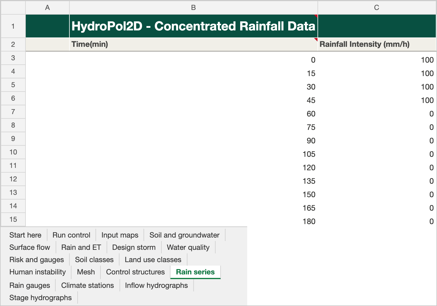
The Rain series tab of the Stanford example workbook. Click the picture to open it full size.

Uniform series

The Rain series tab holds one gauge: rainfall intensity (mm/h) over time. The rain is applied uniformly over the domain. The tab is read when rainfall is on and no design storm, map, satellite or spatial rainfall is chosen.

Each time starts an interval. A value holds until the next time; the last value holds for one more interval, and then the rate is 0. In the V-tilted example, 10.8 mm/h at 0 min and 0 mm/h at 90 min mean rain at 10.8 mm/h from 0 to 90 min and none from 90 to 180 min. The same rule applies to rain gauges, rainfall maps, evaporation and transpiration maps and inflow hydrographs. A stage hydrograph holds each depth from its time to the next.

Changed on 2026-10-29

Before 2026-10-29, MATLAB read the times of rain, inflow and ET maps as interval ends, and HydroPol2D-Python read them as interval starts. MATLAB now reads them as interval starts too. The first row of a table that starts at 0 min, as every date-based table does, is now used. A table written with interval ends (first time = one step) must move each time one step earlier to keep its meaning. Design storms are restamped automatically.

Rain gauges

The Rain gauges tab holds several gauges, interpolated to every cell by inverse distance weighting. It is read when flag_spatial_rainfall = 1 and no rainfall maps are given. Each gauge is one column: its index, name and coordinates (m, in the DEM projection), then its intensity (mm/h) at each time (min) of column B.

The Rain gauges tab of the Stanford example workbook. Click the picture to open it full size. The Stanford case does not use this tab; it keeps the template's columns.

Rainfall maps

The Rainfall maps list on the Rain and ET tab has one row per map: the time in minutes since the start date and the path of a GeoTIFF in mm/h. It is read when flag_input_rainfall_map = 1 or a satellite rainfall switch is 1.

---

Design Storms

The Design storm tab generates a synthetic hyetograph instead of reading a rainfall series:

Setting	Key	Unit
Alternated blocks or Huff curves	flag_alternated_blocks, flag_huff	0 / 1
Return period	RP	years
Storm duration	Rainfall Duration	min
Hyetograph time step	dt_design	min
IDF coefficients	K, a, b, c	see below

The intensity follows the local IDF relation

$$i = \frac{K\,\mathrm{RP}^{a}}{(b + t_d)^{c}}$$

where $i$ is the intensity (mm/h), $\mathrm{RP}$ the return period (years) and $t_d$ the duration (min). $K$ must be consistent with these units; $a$ and $c$ are dimensionless and $b$ is in minutes. Use coefficients fitted for the study location.

---

Evapotranspiration

Penman–Monteith from climate stations

With flag_ETP = 1 and no ET maps, HydroPol2D computes evapotranspiration with Penman–Monteith from daily weather at one or more stations, interpolated to the grid by inverse distance weighting. On the Climate stations tab, row 2 names each station block (index, easting and northing in m), row 3 heads its columns, and each row from row 4 is one day. Typical variables are air temperature, radiation, relative humidity and wind speed.

The Climate stations tab of the Stanford example workbook. Click the picture to open it full size. The Stanford case does not use this tab; it keeps the template's columns.

Evaporation and transpiration maps

With flag_input_ETP_map = 1, the model reads two lists on the Rain and ET tab, Transpiration maps and Evaporation maps. Each row is the time in days since the start date and the path of a GeoTIFF in mm/day. Both lists must have the same times. The fluxes are applied directly to surface water and soil moisture, so no meteorological forcing is needed.

Fixed on 2026-10-20

In General_Data.xlsx the rainfall, transpiration and evaporation lists share one header row. Before 2026-10-20, the transpiration list read the rainfall list's Time [min] column (with no day-to-minute conversion), and the evaporation list read the transpiration paths. Runs with flag_input_ETP_map = 1 made before that date used wrong ET times and evaporation maps. Rerun those cases. Each list now stops at its first empty row, and its columns are searched only under its own title, in both layouts.

---

Boundary Hydrographs

Inflow hydrographs

The Inflow hydrographs tab, read when flag_inflow = 1, holds up to 50 gauges. Each gauge is a block of five columns: time (min), flow (m³/s), and the easting and northing (m) of each cell the flow enters, one cell per row. The flow is spread over those cells. Keep all 50 blocks, even empty ones.

The Inflow hydrographs tab of the Stanford example workbook. Click the picture to open it full size. The Stanford case does not use this tab; the template's gauge names are left out of the picture.

Inflow hydrographs represent upstream boundaries, river inflow, and dam-break or controlled releases.

Stage hydrographs

The Stage hydrographs tab, read when flag_stage_hydrograph = 1, has the same layout: time (min), water depth (m), and the easting and northing (m) of each boundary cell. All cells of a boundary receive the same imposed depth. Keep all 50 blocks, even empty ones.

The Stage hydrographs tab of the Stanford example workbook. Click the picture to open it full size. The Stanford case does not use this tab; it keeps the template's columns.

Stage hydrographs represent downstream control, backwater and other hydraulic constraints.

---

Practical Considerations

• Keep all forcing in the same time reference as date_begin and date_end.
• Check the units of each series: rainfall in mm/h, ET maps in mm/day, inflow in m³/s, stage in m.
• Do not mix rainfall sources, and check that gauges and boundary cells are placed in the DEM projection.
• Use a forcing interval that resolves the peaks you need, given the model time step.

---

Older Layout

In cases that use General_Data.xlsx, each series is its own workbook in the same folder: Rainfall_Intensity_Data.xlsx (Rain series), Rainfall_Spatial_Input.xlsx (Rain gauges), ETP_input_data.xlsx (Climate stations), Inflow_Hydrograph.xlsx and Stage_Hydrograph.xlsx. The map lists are the Satellite or Radar Rainfall, Satellite transpiration and Satellite evaporation tables of General_Data. The case workbook keeps the same cell layout, so the model reads both layouts the same way.