Preview and cost
Preview domain and cost draws the domain and estimates the size of the case in seconds, before any large download. Nothing is built yet, so you can change the settings and preview again until the domain is right. Prepare complete case stays greyed out until the preview matches the current settings.
Before the preview
Above the two buttons, the page checks the request:
- the period each rainfall source has, for example "NASA IMERG Final Run availability: 1998-01-01 through 2025-09-30";
- the accounts and tools the case needs. When one is missing, a yellow box says "This case cannot be prepared yet:" and names it (see Data sources and accounts);
- for AORC, that the whole domain lies inside the AORC grid, which the preview confirms;
- when everything is in place: "Required credentials, source coverage, and local tools are ready for this request."
What the preview shows
- Case files: the folder of the case, in green. The preview already writes the request, the domain and the preview maps there.
- The domain on a map. The map is interactive, over OpenTopoMap. The layer control switches to a street map or hides the overlays. The online map is only a background: it does not change the case.
- Estimated quadtree grid (quadtree cases): the resolution zones of the mesh.
- Rivers entering the domain (Urban Area Only): see Choose the model area.
- The size of the case: six numbers, and for a quadtree grid the cells of each size.
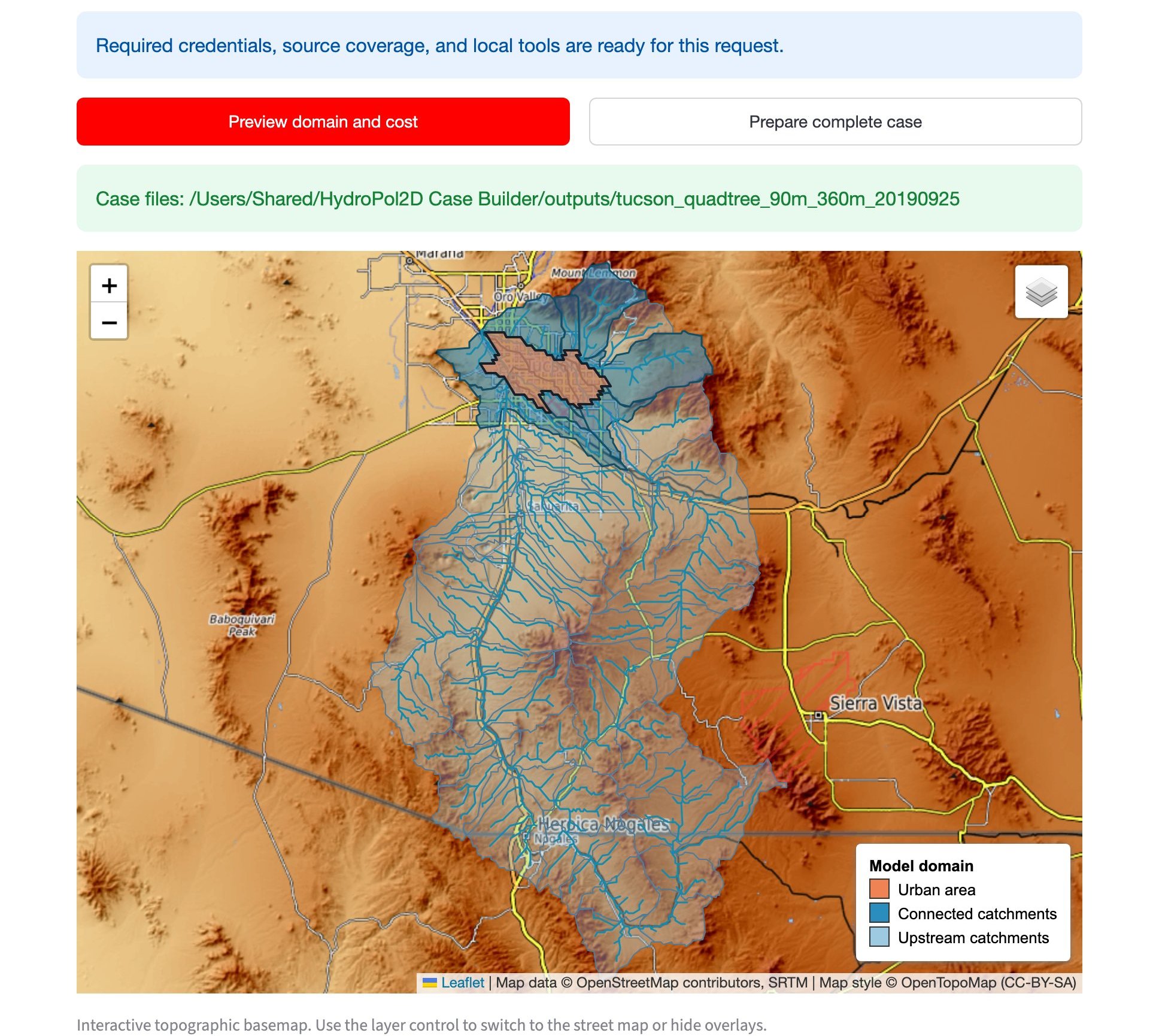
Figure 1. The preview of the Tucson urban basin. The city (orange) lies downstream in the Santa Cruz River basin, so the upstream catchments reach south across the border into Mexico.
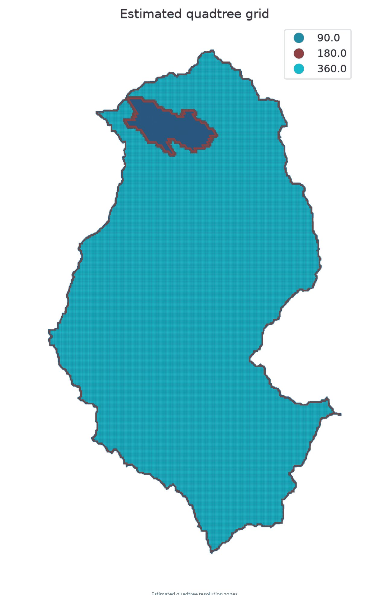
Figure 2. The quadtree zones of the same case: 90 m cells over the city and its buffer, a band of 180 m cells, and 360 m cells over the rest of the basin.
For a Catchment case, the map shows the outlet you entered, the three candidate outlets on the river network and a first outline of the catchment.
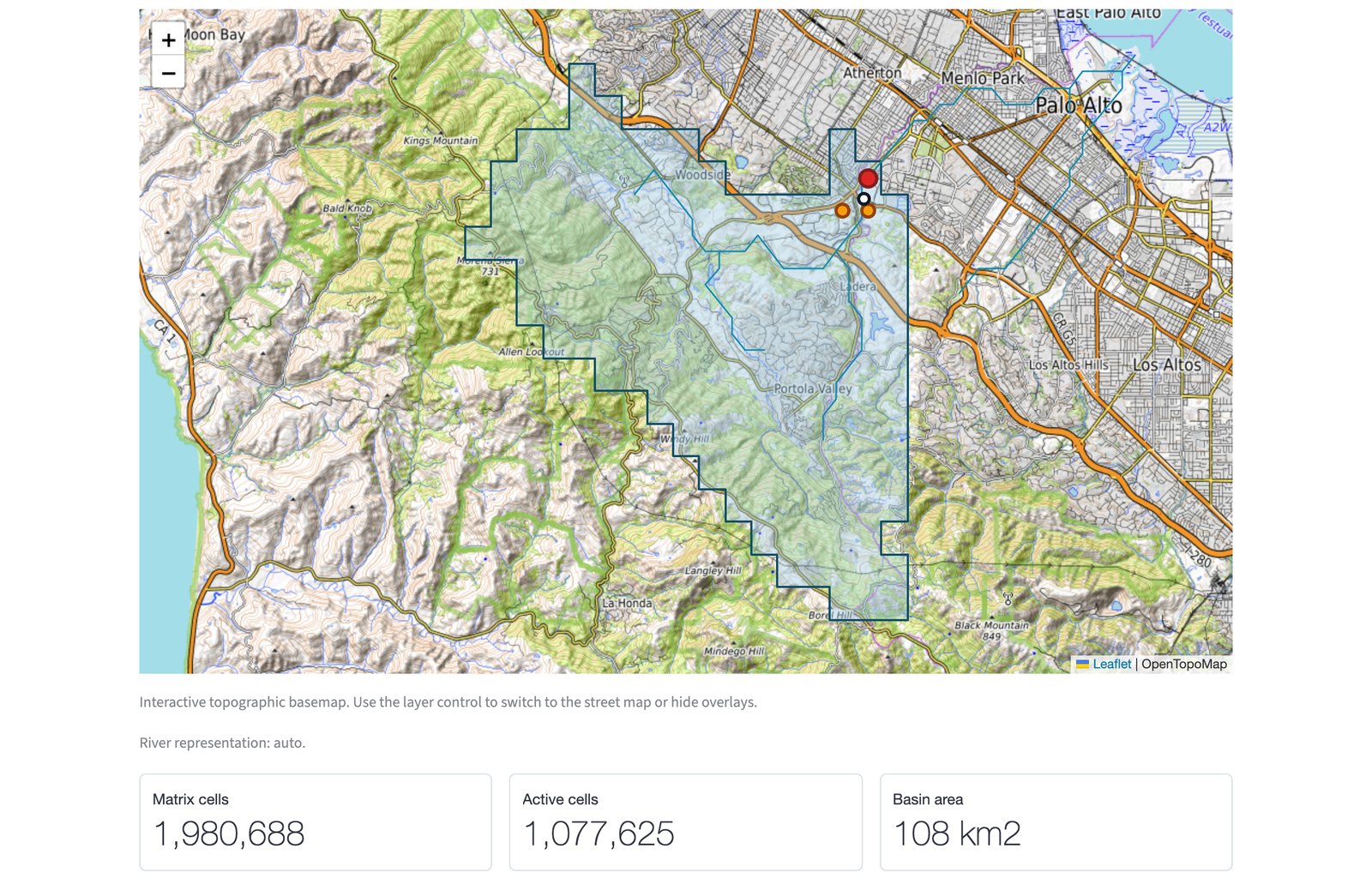
Figure 3. The preview of San Francisquito Creek. The red dot is the outlet you entered, the orange dots are the candidate outlets, and the outline is a first sketch of the catchment. The complete build delineates the catchment again on the model grid.
The size of the case
| Number | What it means |
|---|---|
| Matrix cells | rows times columns of the rectangle around the whole domain |
| Active cells | the cells inside the domain |
| Basin area | the area of the domain, in km² |
| Temporary transfer ceiling | an upper bound of the source data the build downloads, static maps and forcing together |
| Retained forcing inputs | the rain and weather kept with the finished case |
| Estimated saved outputs | the size of the results the model will save, from the outputs you chose |
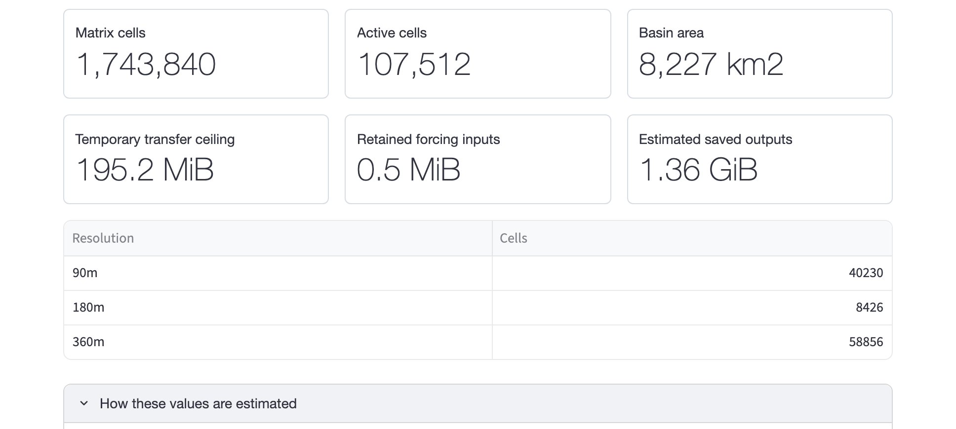
Figure 4. The size of the Tucson case: 107,512 active cells on a 8,227 km² basin, under 200 MiB to download and about 1.4 GiB of results.
Memory depends mostly on the matrix, not only on the active cells. A long or broken-up domain can need more memory than its area suggests. How these values are estimated explains each number and lists the download and the saved outputs by source. Some notes from it:
- The transfer counts the source values at each product's own resolution, over the domain and the period. It does not count the HydroPol2D rasters the build writes. MSWEP is counted as uncompressed values, so the real traffic is lower.
- Raw source files are removed after a successful build. A failed build keeps them, so the next attempt resumes.
- The saved-output estimate counts the selected files only, as uncompressed values.
Start large regional models at a coarse cell size, read the numbers, and go finer only when they fit your computer.
When the settings change
Any change after a preview shows "Settings changed. Run the preview again before preparing this case." The Process log at the bottom of the tab keeps the messages of the last preview or build.