San Francisquito Catchment - 10 m LiDAR Controlled Event

Purpose

This example presents the San Francisquito 10 m LiDAR simulation. It shows how the model responds when the terrain is represented with a finer DEM.

Case setup

The 10 m example uses:

• a real 10 m USGS or 3DEP DEM for the Stanford domain;
• ancillary Stanford rasters aligned to that 10 m grid;
• the same controlled rainfall event used in the 30 m example;
• a perimeter outlet treatment.

Item	Value
Grid resolution	10 m
Forcing	100 mm/h for 1 hour
Simulation duration	6 h
Map output interval	15 min
Saved map frames	24
Routing family	Local inertial
Outlet treatment	Perimeter outlet

Simulation video

The animation below shows the 10 m simulation. The panels show flood depth, velocity, hazard metric, and cumulative infiltration.

San Francisquito 10 m LiDAR simulation: flood depth, velocity, hazard, and cumulative infiltration over six hours.

Six-hour response summary

The summary below refers to the same six-hour simulation shown in the map sequence.

Metric	Value
Grid resolution	10 m
Published duration	6 h
Saved map frames	24
Map sequence covered	00:00 to 05:45
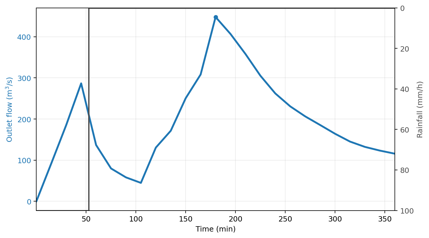
Peak outlet flow in the six-hour window	448.06 m³/s
Peak timing	180.00 min
Outlet flow at 6 h	115.69 m³/s
Maximum saved-frame depth	6.91 m
Maximum saved-frame velocity	10.00 m/s
Maximum saved-frame hazard metric	25.38 m²/s
Maximum cumulative infiltration	474.60 mm

Hydrograph and rainfall

What this example shows

This example highlights:

• the effect of a finer terrain representation on local inundation patterns;
• the early routed response during the first six simulation hours;
• the differences that emerge when the same forcing is applied on the 10 m and 30 m domains.