Downloads
📋 Excel Workbook
X-WHAT_Model_V1.5.xlsm, the core engine with the
Memory, Mass_Balance, and Energy_Balance sheets.
📕 PDF User Manual
The complete manual with all tutorials, parameter tables, worked examples, and troubleshooting, formatted for print.
Download PDF ↓📄 Theoretical Framework
The governing equations, the cost model, and the two optimization problems, with the link to the publication.
Read the theory →The Workflow
X-WHAT pairs a web interface with an Excel engine. The web pages prepare the inputs and visualize the outputs, while every hydraulic calculation runs inside the open spreadsheet through the built-in Solver. No coding is required at any point.
Draw the Network
Place junctions, tanks, pipes, and loops in the Network Builder, or load a tutorial case.
Set the Mode
Choose WFP/HSP for simulation or DOM for cost optimization, then review demands, heads, and boundary conditions.
Export the Package
Download the .xwhat.xml file holding all node data,
geometry, matrices, and parameters.
Import into Excel
Open X-WHAT_Model_V1.5.xlsm, enable macros, and run
Import Network to fill every input cell.
Run the Solver
Configure the GRG Nonlinear Solver for your analysis mode, solve, and save the workbook.
Tutorials
Each tutorial covers one stage of the workflow and they are meant to be followed in order on a first use. Every tutorial opens with a video version and then gives the same material in written form, with annotated steps and short notes on common mistakes.
Tutorial 1
Building a Network in the Network Builder
+
The Network Builder is an interactive canvas where the topology and the input data of the model are defined. The toolbar on the left holds the drawing tools, the panel on the right edits the properties of the selected element, and the top bar gives access to the project settings, the analysis mode, and the workflow roadmap.
| Tool | Shortcut | Purpose |
|---|---|---|
| Select | S | Select and drag elements, edit their properties |
| Pan | H | Move the view around the canvas |
| Junction | J | Place demand nodes |
| Tank | T | Place tanks and reservoirs |
| Pipe | P | Connect two nodes with a link |
| Loop | L | Group pipes into a closed loop |
| Delete | Del | Remove the clicked element |
-
Place the nodes
Activate the Junction tool and click the canvas to place each junction. Use the Tank tool for reservoirs and tanks. Nodes receive a continuous numbering in the order of creation.
Sketch the system on paper first and reproduce a similar layout on the canvas. A clean drawing makes the loops easier to trace and the results easier to interpret. -
Connect the pipes
Activate the Pipe tool, click the upstream node, then click the downstream node. The drawing order defines the positive flow direction of the pipe. To fix a pipe drawn backwards, select it and press Reverse Direction in the properties panel.
-
Edit the element properties
With the Select tool, click any element and fill its fields in the right panel. Junctions take an elevation in meters and a demand in L/s, positive when water leaves the network at that node. Pipes take a length, a diameter, and the friction data of the chosen model, the roughness for Darcy-Weisbach or the coefficient C for Hazen-Williams.
Tanks additionally take the headhrabove the ground, the tower heighthb, and the pump data, daily working hours, efficiency, and the head loss coefficientkpof the supply line. -
Define the loops
Activate the Loop tool and click, one by one, the pipes that close each loop, following the clockwise convention. Every independent loop of the network must be defined because the loops generate the energy balance matrix.
Open Matrix Preview at the bottom of the screen to inspect the incidence matrices produced by the drawing. Checking them before the export saves a round trip to Excel. -
Set the boundary conditions
Every tank requires a fixed head. A junction with known pressure can also be fixed by ticking Fixed Head Node in its properties and typing the pressure head in meters.
-
Choose the analysis mode
In the top bar, keep Mode: WFP / HSP for a hydraulic simulation or switch to Mode: DOM (Optimization) for a cost optimization. The mode is stored in the exported package and adjusts the guidance shown in the Roadmap.
-
Review the project settings
Open Settings to define the global parameters, the friction method, the fluid properties, the energy price, the interest and energy increase rates, the demand factors, the wind data, and the pipe cost catalog. Default values suitable for a first run are already loaded.
-
Export the network package
Press Export Network Package and keep the recommended
.xwhat.xmlformat. The file carries the node table, the pipe geometry, both incidence matrices, and the global parameters, ready for the workbook import.Save JSON stores an editable copy of the drawing itself. Load it back later with Load JSON to continue the work where it stopped.
Tutorial 2
Running a Hydraulic Simulation (WFP/HSP) in Excel
+
The Water Flow Problem determines the discharge and the direction of flow in every pipe of a network with known diameters and fixed tank heads. The Solver searches a flow vector that closes the mass balance at all nodes and the energy balance in all loops, with no objective function involved.
-
Open the workbook and enable macros
Open
X-WHAT_Model_V1.5.xlsmand click Enable Content in the security bar. The macro is used only by the import feature. The hydraulic model itself runs on regular worksheet formulas. -
Import the network package
Click Import Network and select the
.xwhat.xmlfile exported from the Network Builder. The Memory, Mass_Balance, and Energy_Balance sheets are populated automatically.White cells receive user input and gray cells hold automatic calculations. After importing, sweep the white cells once to confirm the data arrived as expected. -
Open the Solver
Go to Data and click Solver. If the command is missing, enable the Solver Add-in following the FAQ at the bottom of this page.
-
Configure the Solver
For a network with P links, N nodes, and L loops, the setup is
Set Objective: leave blank (feasibility search) Changing Cells: Memory!AI50:AI(49+P) pipe discharges q Constraints: Memory!BE51:BE(50+N) = 0 mass balance residuals Memory!BH51:BH(50+L) = 0 energy balance residuals Method: GRG NonlinearAs a concrete example, the Huddleston (2004) tutorial network has 21 links, 14 nodes, and 8 loops, which gives the ranges
AI50:AI70,BE51:BE64, andBH51:BH58.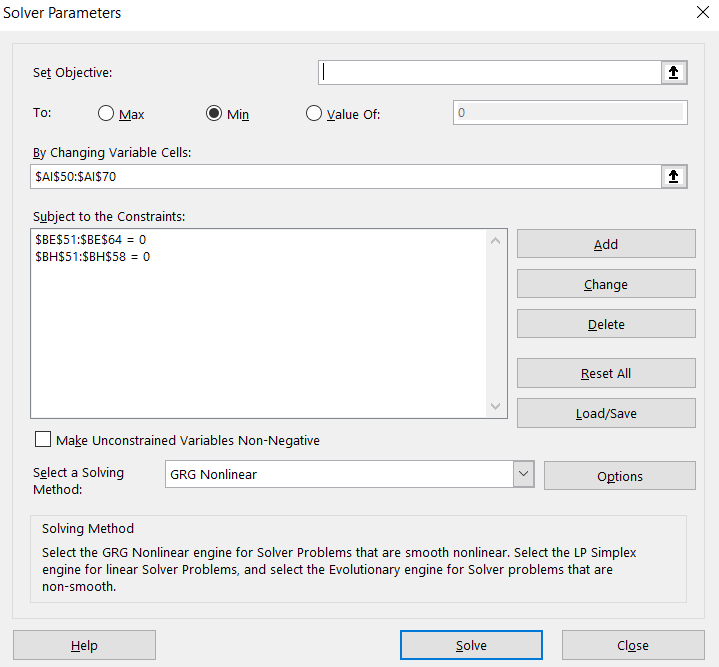
Solver window for the Huddleston (2004) case in WFP mode. With a tutorial network loaded, the Roadmap window in the Network Builder prints the exact ranges for that case, so they can be copied straight into the Solver dialog. -
Solve and verify the convergence
Click Solve. When the Solver reports that all constraints are satisfied, accept the solution and inspect the flow column. Confirm that the residuals in
BEandBHare effectively zero and that the flow directions are physically sensible.If the Solver stops before converging, run it again from the current values, or enable Multistart in the GRG options. Distant initial flow values are the most common cause of early stops. -
Save the solved workbook
Save with Ctrl + S. The saved file feeds the Results page, covered in Tutorial 4.
Tutorial 3
Running a Design Optimization (DOM) in Excel
+
Design Optimization Modeling extends the simulation by letting the Solver adjust design variables, typically the tank water depths and tower heights, in search of the lowest total cost. The objective gathers pipelines, pumping energy in present value, tank material, and the foundation under wind loading, while every nodal pressure must stay inside the allowed band.
-
Prepare the network in DOM mode
In the Network Builder, switch the selector to Mode: DOM (Optimization) before exporting. In this mode the tank heads and tower heights typed in the properties panel act as starting values, so give them reasonable initial estimates.
-
Complete the economic parameters
A DOM run uses the full parameter set of the project settings, the energy price, the interest and energy increase rates, the lifespan, the demand factors, the tank material cost, the design wind speed with its exponent, and the pipe cost catalog. These fields map one to one onto the parameter block of the Memory sheet.
-
Import and audit the cost cells
Import the package as in Tutorial 2 and check that the cost cells of the Memory sheet react to the imported parameters. The total cost in
Memory!BT51gathers the pipeline, pumping, tank material, and foundation components. -
Configure the Solver
Set Objective: Memory!BT51 (Min) total network cost Changing Cells: Memory!AI50:AI(49+P) pipe discharges q tank head cells (col AA) and tower heights (col T) Constraints: Memory!BE51:BE(50+N) = 0 mass balance residuals Memory!BH51:BH(50+L) = 0 energy balance residuals pressure heads (col BK) between p_min and p_max Method: GRG NonlinearIn the audited Huddleston (2004) DOM case, the changing cells are
AI50:AI70,AA63, andT62:T63, with the pressuresBK51:BK62bounded between 10 and 30 m, the tank head above 5 m, and the tower heights between 0 and 39.5 m. The head of the second reservoir stays formula-linked 3.66 m above the first one.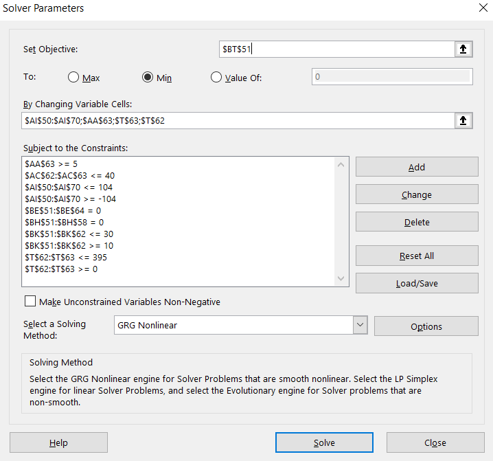
Solver window for the Huddleston (2004) case in DOM mode. -
Solve, restart, and compare
The DOM problem is non-convex, so a single run may land on a local minimum. Solve several times from different starting points, or activate Multistart in the GRG options, record the objective of each run, and keep the best design.
A useful benchmark is the standard design cost, obtained by running the same network in WFP mode with manually chosen tank depths. In the paper, the optimization of case (c) cut the total cost by 151,790 USD, about 9.8%. -
Save the solved workbook
Save the file and continue to Tutorial 4 to visualize the optimized design.
Tutorial 4
Visualizing Results in the Results Viewer
+
The Results page reads a solved workbook directly in the browser and mounts an interactive dashboard. The file is processed locally by the page, nothing is sent to a server.
-
Upload the solved workbook
Drag the saved
.xlsmor.xlsxfile onto the upload area, or click Choose Solved Workbook and browse to it. -
Read the flow diagram
The Network Flow tab draws the network with the pipe width proportional to the flow magnitude. Blue pipes follow the drawn direction and red pipes carry reversed flow.
-
Check the node pressures
The Node Pressures tab lists the head and the pressure at every node. Confirm that all values sit inside the design band, commonly 10 to 30 mH2O for distribution networks.
-
Inspect the link flows
The Link Flows tab tabulates each pipe with its length, diameter, discharge, direction, and cost, a convenient format for reports and for comparisons with EPANET.
-
Analyze the cost breakdown
The Cost Breakdown tab splits the total cost into pipelines, pumping energy, tank material, and foundation. In DOM studies this chart is the natural place to compare candidate designs.
Tutorial 5
Using the Excel Engine Directly (Manual Data Entry)
+
The workbook can also be filled entirely by hand, with no help from the Network Builder. This path suits the classroom especially well, because typing the incidence matrices consolidates the understanding of network topology. The workbook holds three sheets. Memory receives the parameters and the element tables, Mass_Balance receives the node incidence matrix, and Energy_Balance receives the loop incidence matrix.
-
Define the global parameters
At the top of the Memory sheet, choose the head loss method, D-W for Darcy-Weisbach or H-W for Hazen-Williams, and type the number of links, nodes, and loops. These three counts size every table and matrix in the workbook. For a plain simulation, the counts and the fluid properties are enough. The remaining parameters serve the cost model in DOM runs.
Parameter Description νKinematic viscosity of the fluid in m²/s ρDensity of the fluid in kg/m³ Links, Nodes, LoopsTotals of the network, they size all tables PcEnergy price in USD/kWh irAnnual increase rate of the energy price YearsLifespan of the system in years RateInterest rate of the project αOperational cost rate for maintenance and operation k1,k2Day and hour demand factors DtrDuration to fill the reservoir, in days Material CostTank material cost per square meter Vk,pDesign wind speed and wind profile exponent -
Enter the node data
For each node, type the ground elevation and select the type, Manhole or Reservoir/Tank. Type the demand in L/s, positive when water is withdrawn. Set the Fixed Head flag to 1 for nodes with a pressure boundary condition and type the pressure head. Every node marked as Reservoir/Tank requires a fixed head.
-
Enter the tank and pump data
In the rows marked as Reservoir/Tank, type the bottom elevation, the height above the ground, and the pump data, daily working hours, efficiency, pump elevation, and the head loss coefficient of the supply line. The sheet then computes the pump flow, the manometric head, the power, and the daily and annual energy costs.
-
Enter the link data
For each link, pick the upstream and downstream nodes from the dropdown lists and type the length and the internal diameter. The pipe cost is evaluated automatically by the fitted cost function. The flow column is the decision variable, so any initial guess can be typed there.
-
Fill the mass balance matrix
In the Mass_Balance sheet, each row is a node and each column is a link. Type +1 where the pipe enters the node, -1 where the pipe leaves it, and 0 elsewhere. For instance, a node fed by pipe 20 that discharges through pipes 1 and 9 receives +1 in column 20 and -1 in columns 1 and 9, with zeros in the rest of the row.
-
Fill the energy balance matrix
In the Energy_Balance sheet, each row is a loop and each column is a link. Type +1 when the pipe direction agrees with the clockwise circulation of the loop, -1 when it opposes it, and 0 when the pipe does not belong to the loop.
The matrix dimensions follow the totals declared in step 1, so always define the counts first and the matrices last. -
Run the Solver
Follow Tutorial 2 for a simulation or Tutorial 3 for an optimization. The Solver setup is identical regardless of how the data entered the workbook.
Troubleshooting and FAQ
The Solver stops without finding a solution
Excel blocks the macros when the workbook opens
Some discharges come out negative
The mass balance never closes at one specific node
Which head loss model should I pick?
The Solver command is missing from the Data tab
Can I modify the cost functions or the objective?
How large can the network be?
For Educators
X-WHAT was designed with the classroom in mind. Every formula is exposed in the spreadsheet, so students can trace how the conservation laws, the friction models, and the cost functions interact, an insight that closed simulation packages rarely offer. The tutorial cases reproduce networks from the literature and give instructors ready-made exercises with audited answers.
The publication also proposes a complete class organization following the Understanding by Design (UbD) framework, with learning goals, essential questions, assessment evidence, and a suggested sequence of activities built around the model. See the paper and its supplemental material on the Theoretical Framework page.